Deep learning neural network case (handwritten digit recognition)

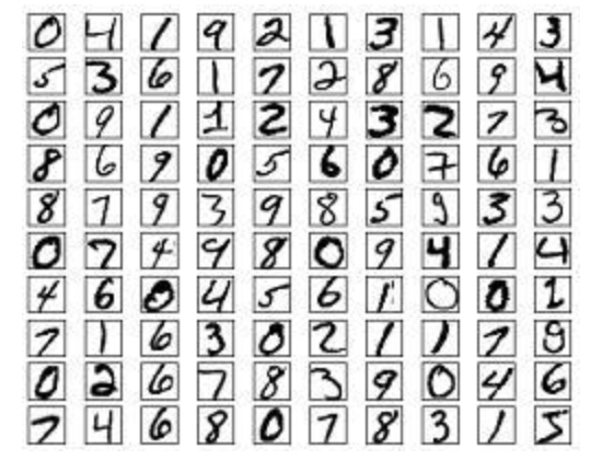
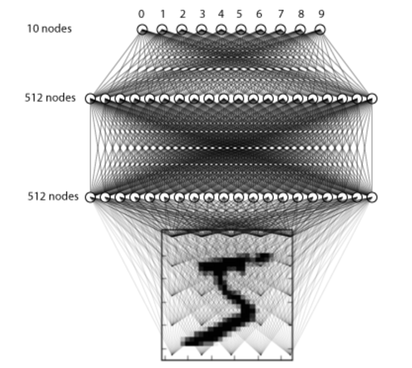
Using handwritten numerals MNIST The data set is shown in the figure above , The dataset contains 60,000 Samples for training and 10,000 A sample for testing , The image is a fixed size (28x28 Pixels ), Its value is 0 To 255.

The implementation process of the whole case is ：

• Data loading
• Data processing
• model building
• model training
• Model test
• Model preservation

First, import the required toolkit ：

#  Import the corresponding toolkit 
import numpy as np
import matplotlib.pyplot as plt
plt.rcParams['figure.figsize'] = (7,7) # Make the figures a bit bigger
import tensorflow as tf
#  Data sets 
from tensorflow.keras.datasets import mnist
#  Build a sequence model 
from tensorflow.keras.models import Sequential
#  Import the required layers 
from tensorflow.keras.layers import Dense, Dropout, Activation,BatchNormalization
#  Import the auxiliary Kit 
from tensorflow.keras import utils
#  Regularization 
from tensorflow.keras import regularizers

1. Data loading

First, load the handwritten digital image

#  Total categories 
nb_classes = 10
#  Load data set 
(X_train, y_train), (X_test, y_test) = mnist.load_data()
#  Print out the dimensions of the dataset 
print(" Initial dimension of training sample ", X_train.shape)
print(" Initial dimension of target value of training sample ", y_train.shape)

The result is ：

 Initial dimension of training sample  (60000, 28, 28)
 Initial dimension of target value of training sample  (60000,)

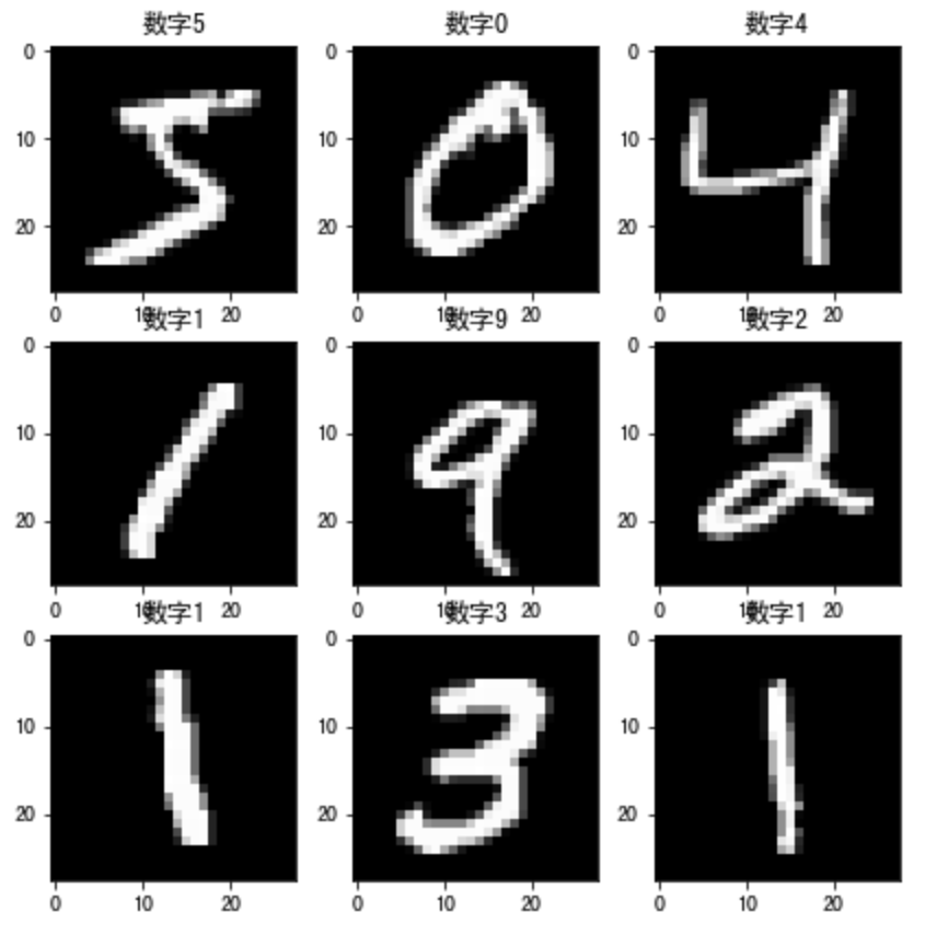
Data presentation ：

#  Data presentation ： Show the first nine data sets of the data set 
for i in range(9):
    plt.subplot(3,3,i+1)
    #  Display in grayscale , No interpolation 
    plt.imshow(X_train[i], cmap='gray', interpolation='none')
    #  Set the title of the picture ： Corresponding category 
    plt.title(" Numbers {}".format(y_train[i]))

The effect is as follows ：

2. Data processing

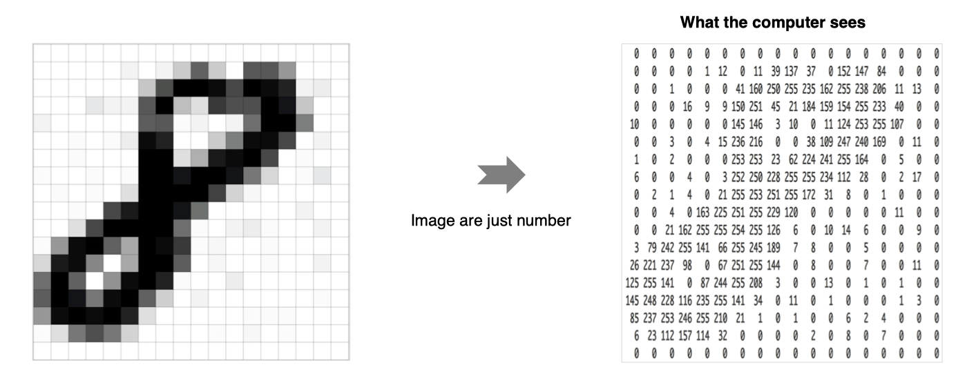
Each training sample in the neural network is a vector , Therefore, the input needs to be reshaped , Make each 28x28 The image becomes a 784 Dimension vector . in addition , Normalize the input data , from 0-255 To adjust to 0-1.

#  Adjust data dimension ： Each number is converted into a vector 
X_train = X_train.reshape(60000, 784)
X_test = X_test.reshape(10000, 784)
#  format conversion 
X_train = X_train.astype('float32')
X_test = X_test.astype('float32')
#  normalization 
X_train /= 255
X_test /= 255
#  Dimension adjusted results 
print(" Training set ：", X_train.shape)
print(" Test set ：", X_test.shape）

Output is ：

 Training set ： (60000, 784)
 Test set ： (10000, 784)

In addition, we also need to deal with the target value , Convert it to hot coded form ：

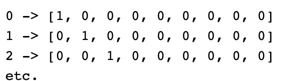
The implementation is as follows ：

#  Convert the target value to a hot coded form 
Y_train = utils.to_categorical(y_train, nb_classes)
Y_test = utils.to_categorical(y_test, nb_classes)

3. model building

Here we build only 3 Layer fully connected network for processing ：

The construction method is as follows ：

#  Use the sequence model to build the model 
model = Sequential()
#  Fully connected layer , common 512 Neurons , The input dimension size is 784
model.add(Dense(512, input_shape=(784,)))
#  Activate function using relu
model.add(Activation('relu')) 
#  Using the regularization method drouout 
model.add(Dropout(0.2))  
#  Fully connected layer , common 512 Neurons , And add L2 Regularization 
model.add(Dense(512,kernel_regularizer=regularizers.l2(0.001)))
# BN layer 
model.add(BatchNormalization())
#  Activation function 
model.add(Activation('relu'))
model.add(Dropout(0.2))
#  Fully connected layer , Output layer total 10 Neurons 
model.add(Dense(10))
# softmax The output of neural network score Convert to probability value 
model.add(Activation('softmax')) 

We go through model.summay Look at the results ：

Model: "sequential_6"
_________________________________________________________________
Layer (type)                 Output Shape              Param # 
=================================================================
dense_13 (Dense)             (None, 512)               401920    
_________________________________________________________________
activation_8 (Activation)    (None, 512)               0         
_________________________________________________________________
dropout_7 (Dropout)          (None, 512)               0         
_________________________________________________________________
dense_14 (Dense)             (None, 512)               262656    
_________________________________________________________________
batch_normalization (BatchNo (None, 512)               2048      
_________________________________________________________________
activation_9 (Activation)    (None, 512)               0         
_________________________________________________________________
dropout_8 (Dropout)          (None, 512)               0         
_________________________________________________________________
dense_15 (Dense)             (None, 10)                5130      
_________________________________________________________________
activation_10 (Activation)   (None, 10)                0         
=================================================================
Total params: 671,754
Trainable params: 670,730
Non-trainable params: 1,024
_________________________________________________________________

4. Model compilation

Set the loss function used in model training, cross entropy loss and optimization method adam, The loss function is used to measure the difference between the predicted value and the real value , The optimizer is used to achieve optimization using the loss function ：

#  Model compilation , Indicate the loss function and optimizer , Evaluation indicators 
model.compile(loss='categorical_crossentropy', optimizer='adam',metrics=['accuracy'])

5. model training

# batch_size Is the number of samples sent into the model each time ,epochs Is the number of iterations of all samples , And indicate the validation data set 
history = model.fit(X_train, Y_train,
          batch_size=128, epochs=4,verbose=1,
          validation_data=(X_test, Y_test))

The training process is as follows ：

Epoch 1/4
469/469 [==============================] - 2s 4ms/step - loss: 0.5273 - accuracy: 0.9291 - val_loss: 0.2686 - val_accuracy: 0.9664
Epoch 2/4
469/469 [==============================] - 2s 4ms/step - loss: 0.2213 - accuracy: 0.9662 - val_loss: 0.1672 - val_accuracy: 0.9720
Epoch 3/4
469/469 [==============================] - 2s 4ms/step - loss: 0.1528 - accuracy: 0.9734 - val_loss: 0.1462 - val_accuracy: 0.9735
Epoch 4/4
469/469 [==============================] - 2s 4ms/step - loss: 0.1313 - accuracy: 0.9768 - val_loss: 0.1292 - val_accuracy: 0.9777

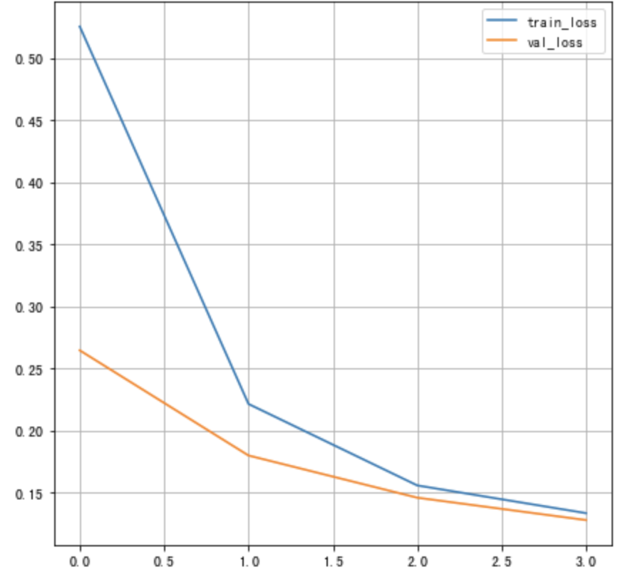
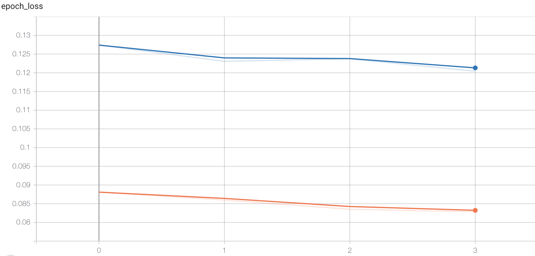
Draw the loss curve ：

#  Draw the change curve of the loss function 
plt.figure()
#  Training set loss function transformation 
plt.plot(history.history["loss"], label="train_loss")
#  Verification set loss function change 
plt.plot(history.history["val_loss"], label="val_loss")
plt.legend()
plt.grid()

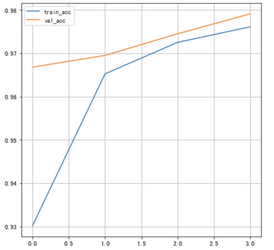
Draw the training accuracy as a curve ：

#  Draw the change curve of accuracy 
plt.figure()
#  Training set accuracy 
plt.plot(history.history["accuracy"], label="train_acc")
#  Verification set accuracy 
plt.plot(history.history["val_accuracy"], label="val_acc")
plt.legend()
plt.grid()

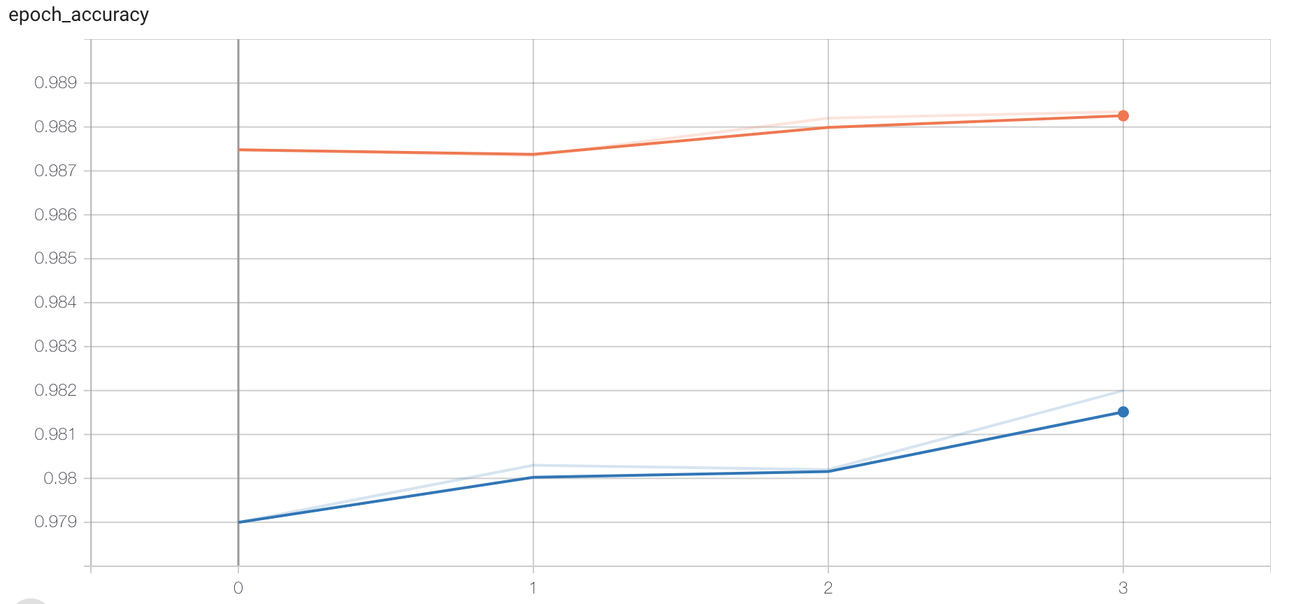
In addition, through tensorboard Monitor the training process , At this point, we specify the callback function ：

#  add to tensoboard Observe 
tensorboard = tf.keras.callbacks.TensorBoard(log_dir='./graph', histogram_freq=1,
                                                write_graph=True,write_images=True)

In training ：

#  Training 
history = model.fit(X_train, Y_train,
          batch_size=128, epochs=4,verbose=1,callbacks=[tensorboard],
          validation_data=(X_test, Y_test))

Open the terminal ：

#  Specify the directory where the file exists , Open the following command 
tensorboard --logdir="./"

Open the specified web address in the browser , You can view the change of loss function and accuracy , Graph structure, etc .

6. Model test

#  Model test 
score = model.evaluate(X_test, Y_test, verbose=1)
#  Print the results 
print(' Test set accuracy :', score)

result ：

313/313 [==============================] - 0s 1ms/step - loss: 0.1292 - accuracy: 0.9777
Test accuracy: 0.9776999950408936

7. Model preservation

#  Save the model structure and weight in h5 In file 
model.save('my_model.h5')
#  Load model ： Including the architecture and corresponding weights 
model = tf.keras.models.load_model('my_model.h5')

summary

• Be able to use tf.keras Get data set ：
  load_data()

• Be able to construct multilayer neural network
  dense, Activation function ,dropout,BN Layer, etc.

• Be able to complete network training and evaluation
  fit, Callback function ,evaluate, Save the model