当前位置:网站首页>《动手学深度学习》(二)-- 多层感知机
《动手学深度学习》(二)-- 多层感知机
2022-07-02 03:44:00 【长路漫漫2021】
1 多层感知机
1.1 从零开始实现
本节将继续使⽤Fashion-MNIST图像分类数据集,数据导入步骤和上一节一样,本节将不再展示。
import torch
from d2l import torch as d2l
import torch.nn.functional as F
from torch.utils.data import DataLoader
from torch.utils import data
from torchvision import transforms
from torch import nn

mnist_train = FashionMnistDataset("../dataset/fashion-mnist", "train-images-idx3-ubyte.gz", "train-labels-idx1-ubyte.gz", transform=transforms.ToTensor())
mnist_test = FashionMnistDataset("../dataset/fashion-mnist", "t10k-images-idx3-ubyte.gz", "t10k-labels-idx1-ubyte.gz", transform=transforms.ToTensor())
train_loader = DataLoader(mnist_train, batch_size=256, shuffle=True, num_workers=4)
test_loader = DataLoader(mnist_test, batch_size=256, shuffle=False, num_workers=4)
1. 初始化模型参数
⾸先,我们将实现⼀个具有单隐藏层的多层感知机,它包含256个隐藏单元。注意,我们可以将这两个变量都视为超参数。通常,我们选择2的若⼲次幂作为层的宽度。因为内存在硬件中的分配和寻址⽅式,这么做往往可以在计算上更⾼效。
⽤⼏个张量来表⽰我们的参数。注意,对于每⼀层我们都要记录⼀个权重矩阵和⼀个偏置向量。跟以前⼀样,我们要为这些参数的损失的梯度分配内存。
num_inputs, num_outputs, num_hiddens = 784, 10, 256
W1 = nn.Parameter(torch.randn(num_inputs, num_hiddens, requires_grad=True) * 0.01)
b1 = nn.Parameter(torch.zeros(num_hiddens, requires_grad=True))
W2 = nn.Parameter(torch.randn(num_hiddens, num_outputs, requires_grad=True) * 0.01)
b2 = nn.Parameter(torch.zeros(num_outputs, requires_grad=True))
params = [W1, b1, W2, b2]
2. 激活函数
def relu(X):
    a = torch.zeros_like(X)
    return torch.max(X, a)
3. 模型
使⽤reshape将每个⼆维图像转换为⼀个⻓度为num_inputs的向量。
def net(X):
    X = X.reshape((-1, num_inputs))
    H = relu([email protected] + b1)
    return ([email protected] + b2)
4. 损失函数
loss = nn.CrossEntropyLoss()
5. 训练
多层感知机的训练过程与softmax回归的训练过程完全相同。可以直接调⽤d2l包的train_ch3函数,将迭代周期数设置为10,并将学习率设置为0.1。
num_epoches, lr = 10, 0.1
optimizer = torch.optim.SGD(params, lr=lr)
d2l.train_ch3(net, train_loader, test_loader, loss, num_epoches, optimizer)

6. 评估模型
d2l.predict_ch3(net, test_loader)

1.2 简洁实现
这里和上一节的softmax回归的简洁实现相比,唯一的区别是这里使用了2个全连接层,第一层是隐藏层,包含256个隐藏单元,并使用ReLU激活函数。
net = nn.Sequential(nn.Flatten(), nn.Linear(784, 256), nn.ReLU(), nn.Linear(256, 10))
def init_weights(m):
    if isinstance(m, nn.Linear):
        nn.init.normal_(m.weight, std=0.01)

net.apply(init_weights)

lr, num_epoches = 0.1, 10
loss = nn.CrossEntropyLoss()
optimizer = torch.optim.SGD(net.parameters(), lr=lr)
d2l.train_ch3(net, train_loader, test_loader, loss, num_epoches, optimizer)

2 多项式回归
本节主要以不同阶数的多项式进行回归实验,从而体会过拟合和欠拟合。
import torch
import numpy as np
import torch
from torch import nn
from d2l import torch as d2l
import math
1. 生成数据集
给定 x x x,使用以下三阶多项式来⽣成训练和测试数据的标签:
y = 5 + 1.2 x − 3.4 x 2 2 ! + 5.6 x 3 3 ! + ϵ where ϵ ∼ N ( 0 , 0. 1 2 ) y=5+1.2 x-3.4 \frac{x^{2}}{2 !}+5.6 \frac{x^{3}}{3 !}+\epsilon \text { where } \epsilon \sim \mathcal{N}\left(0,0.1^{2}\right) y=5+1.2x−3.42!x2+5.63!x3+ϵ where ϵ∼N(0,0.12)
噪声 ϵ \epsilon ϵ项服从均值为0且标准差为0.1的正态分布。在优化的过程中,我们通常希望避免⾮常⼤的梯度值或损失值。这就是我们将特征从 x i x^i xi调整为 x i i ! \frac{x^i}{i!} i!xi的原因,这样可以避免很⼤的i带来的特别⼤的指数值。为训练集和测试集各⽣成100个样本。
max_degree = 20                 # 多项式回归的最大阶数
n_train, n_test = 100, 100      # 训练集和测试接大小
true_w = np.zeros(max_degree)   # 分配大量的空间
true_w[0:4] = np.array([5, 1.2, -3.4, 5.6])

features = np.random.normal(size=(n_train + n_test, 1))
np.random.shuffle(features)
poly_features = np.power(features, np.arange(max_degree).reshape(1, -1))        # 200 * 20 特征矩阵
for i in range(max_degree):
    poly_features[:, i] /= math.gamma(i+1)      # gamma(n) = (n-1)!
    # labels的维度:(n_train+n_test, )
labels = np.dot(poly_features, true_w)
labels += np.random.normal(scale=0.1, size=labels.shape)        # 加上误差
同样,存储在poly_features中的单项式由gamma函数重新缩放,其中 Γ ( n ) = ( n − 1 ) ! \Gamma(n)=(n-1)! Γ(n)=(n−1)!。从⽣成的数据集中查看⼀下前2个样本,第⼀个值是与偏置相对应的常量特征。
# NumPyndarray转换为tensor
true_w, features, poly_features, labels = [torch.tensor(x, dtype=torch.float32) for x in [true_w, features, poly_features, labels]]
features[:2], poly_features[:2, :], labels[:2]

2. 训练和测试
⾸先实现⼀个函数来评估模型在给定数据集上的损失。
def evaluate_loss(net, data_loader, loss):
    """评估给定数据集上模型的损失"""
    metric = d2l.Accumulator(2)     # 损失的总和,样本数量
    for X, y in data_loader:
        out = net(X)
        y = y.reshape(out.shape)
        l = loss(out, y)
        metric.add(l.sum(), l.numel())
    return metric[0] / metric[1]
3. 定义训练函数
def train(train_features, test_features, train_labels, test_labels, num_epoches=400):
    loss = nn.MSELoss(reduction='none')
    input_shape = train_features.shape[-1]
    # 不设置偏置,因为已经在多项式特征中实现了它
    net = nn.Sequential(nn.Linear(input_shape, 1, bias=False))
    batch_size = min(10, train_labels.shape[0])
    train_iter = d2l.load_array((train_features, train_labels.reshape(-1, 1)), batch_size)
    test_iter = d2l.load_array((test_features, test_labels.reshape(-1, 1)), batch_size, is_train=False)
    trainer = torch.optim.SGD(net.parameters(), lr=0.001)
    animator = d2l.Animator(xlabel='epoch', ylabel='loss', yscale='log', xlim=[1, num_epoches], ylim=[1e-3, 1e2], legend=['train', 'test'])
    for epoch in range(num_epoches):
        d2l.train_epoch_ch3(net, train_iter, loss, trainer)
        if epoch == 0 or (epoch+1) % 20 == 0:
            animator.add(epoch+1, (evaluate_loss(net, train_iter, loss), (evaluate_loss(net, test_iter, loss))))
    print('weight:', net[0].weight.data.numpy())
使⽤三阶多项式函数,它与数据⽣成函数的阶数相同。结果表明,该模型能有效降低训练损失和测试损失。学习到的模型参数也接近真实值 w = [ 5 , 1.2 , − 3.4 , 5.6 ] w = [5, 1.2, -3.4, 5.6] w=[5,1.2,−3.4,5.6]。
# 从多项式特征中选择前4个维度,即1,x,x^2/2!,x^3/3!
train(poly_features[:n_train, :4], poly_features[n_train:, :4], labels[:n_train], labels[n_train:])

再看看线性函数拟合,减少该模型的训练损失相对困难。在最后⼀个迭代周期完成后,训练损失仍然很⾼。当⽤来拟合⾮线性模式(如这⾥的三阶多项式函数)时,线性模型容易⽋拟合。
# 从多项式特征中选择前2个维度,即1,x
train(poly_features[:n_train, :2], poly_features[n_train:, :2], labels[:n_train], labels[n_train:])
尝试使⽤⼀个阶数过⾼的多项式来训练模型。在这种情况下,没有⾜够的数据⽤于学到⾼阶系数应该具有接近于零的值。因此,这个过于复杂的模型会轻易受到训练数据中噪声的影响。虽然训练损失可以有效地降低,但测试损失仍然很⾼。结果表明,复杂模型对数据造成了过拟合。

# 从多项式特征中选择所有维度
train(poly_features[:n_train, :], poly_features[n_train:, :], labels[:n_train], labels[n_train:], num_epoches=1500)

3 权重衰减
3.1 高维线性回归
这里的权重衰减也就是对权重加上惩罚项,这里以线性回归为例。
import torch
from torch import nn
from d2l import torch as d2l
1. 生成数据
生成公式如下:
y = 0.05 + ∑ i = 1 d 0.01 x i + ϵ where ϵ ∼ N ( 0 , 0.0 1 2 ) y=0.05+\sum_{i=1}^{d} 0.01 x_{i}+\epsilon \text { where } \epsilon \sim \mathcal{N}\left(0,0.01^{2}\right) y=0.05+i=1∑d0.01xi+ϵ where ϵ∼N(0,0.012)
选择标签是关于输⼊的线性函数。标签同时被均值为0,标准差为0.01⾼斯噪声破坏。为了使过拟合的效果更加明显,我们可以将问题的维数增加到d = 200,并使⽤⼀个只包含20个样本的小训练集。
n_train, n_test, num_inputs, batch_size = 20, 100, 200, 5
true_w, true_b = torch.ones((num_inputs, 1)) * 0.01, 0.05
train_data = d2l.synthetic_data(true_w, true_b, n_train)
train_iter = d2l.load_array(train_data, batch_size)
test_data = d2l.synthetic_data(true_w, true_b, n_test)
test_iter = d2l.load_array(test_data, batch_size, is_train=False)
2. 初始化模型参数
定义⼀个函数来随机初始化模型参数。
def init_params():
    w = torch.normal(0, 1, size=(num_inputs, 1), requires_grad=True)
    b = torch.zeros(1, requires_grad=True)
    return [w, b]
3. 定义L2惩罚项
实现这⼀惩罚最⽅便的⽅法是对所有项求平⽅后并将它们求和。
def l2_penalty(w):
    return torch.sum(w.pow(2)) / 2
4. 训练
def train(lambd):
    w, b = init_params()
    net, loss = lambda X: d2l.linreg(X, w, b), d2l.squared_loss
    num_epoches, lr = 100, 0.003
    animator = d2l.Animator(xlabel='epoches', ylabel='loss', yscale='log', xlim=[5, num_epoches], legend=['train', 'test'])
    for epoch in range(num_epoches):
        for X, y in train_iter:
            # 增加了L2范数惩罚项,
            # ⼴播机制使l2_penalty(w)成为⼀个⻓度为batch_size的向量
            l = loss(net(X), y) + lambd * l2_penalty(w)
            l.sum().backward()
            d2l.sgd([w, b], lr, batch_size)
            if (epoch+1) % 5 == 0:
                animator.add(epoch+1, (d2l.evaluate_loss(net, train_iter, loss), d2l.evaluate_loss(net, test_iter, loss)))
        print('w的L2范数是:', torch.norm(w).item())
我们现在⽤lambd = 0禁⽤权重衰减后运⾏这个代码。注意,这⾥训练误差在减少,但测试误差没有减少,这意味着出现了严重的过拟合。
train(lambd=0)

我们使⽤权重衰减来运⾏代码。注意,在这⾥训练误差增⼤,但测试误差减小。这正是我们期望从正则化中得到的效果。
train(lambd=3)

由于权重衰减在神经⽹络优化中很常⽤,深度学习框架为了便于我们使⽤权重衰减,将权重衰减集成到优化算法中,以便与任何损失函数结合使⽤。此外,这种集成还有计算上的好处,允许在不增加任何额外的计算开销的情况下向算法中添加权重衰减。由于更新的权重衰减部分仅依赖于每个参数的当前值,因此优化器必须⾄少接触每个参数⼀次。
在下⾯的代码中,我们在实例化优化器时直接通过weight_decay指定weight decay超参数。默认情况下,PyTorch同时衰减权重和偏移。这⾥我们只为权重设置了weight_decay,所以偏置参数b不会衰减。
def train_concise(wd):
    net = nn.Sequential(nn.Linear(num_inputs, 1))
    for param in net.parameters():
        param.data.normal_()
    loss = nn.MSELoss(reduction='none')
    num_epoches, lr = 100, 0.003
    # 偏置参数没有衰减
    trainer = torch.optim.SGD([{
    'params': net[0].weight, 'weight_decay': wd}, {
    "params": net[0].bias
    }], lr = lr)
    animator = d2l.Animator(xlabel='epoches', ylabel='loss', yscale='log', xlim=[5, num_epoches], legend=['train', 'test'])
    for epoch in range(num_epoches):
        for X, y in train_iter:
            trainer.zero_grad()
            l = loss(net(X), y)
            l.sum().backward()
            trainer.step()
        if (epoch+1) % 5 == 0:
            animator.add(epoch+1, (d2l.evaluate_loss(net, train_iter, loss), d2l.evaluate_loss(net, test_iter, loss)))

    print('w的L2范数:', net[0].weight.norm().item())
train_concise(0)

train_concise(3)

4 暂退法
4.1 从零开始实现
在标准暂退法正则化中,通过按保留(未丢弃)的节点的分数进⾏规范化来消除每⼀层的偏差。换⾔之,每个中间活性值 h h h以暂退概率 p p p由随机变量 h ′ h' h′替换,如下所⽰:
h ′ = { 0 概率为 p h 1 − p 其他情况 h^{\prime}= \begin{cases}0 & \text { 概率为 } p \\ \frac{h}{1-p} & \text { 其他情况 }\end{cases} h′={ 01−ph 概率为 p 其他情况
根据此模型的设计,其期望值保值不变,即 E [ h ′ ] = h E[h']=h E[h′]=h。
要实现单层的暂退法函数,我们从均匀分布U[0, 1]中抽取样本,样本数与这层神经⽹络的维度⼀致。然后保留那些对应样本⼤于p的节点,把剩下的丢弃。
实现dropout_layer函数,该函数以dropout的概率丢弃张量输⼊X中的元素,如上所述重新缩放剩余部分:将剩余部分除以1.0-dropout。
1. 随机失活
import torch
from torch import nn
from d2l import torch as d2l

def dropout_layer(X, dropout):
    assert 0 <= dropout <= 1
    # 在本情况,所有元素都被抛弃
    if dropout == 1:
        return torch.zeros_like(X)
    # 在本情况中,所有元素都被保留
    if dropout == 0:
        return X
    mask = (torch.rand(X.shape) > dropout).float()
    return mask * X / (1.0 - dropout)
2. 定义模型
定义具有两个隐藏层的多层感知机,每个隐藏层包含256个单元。将暂退法应⽤于每个隐藏层的输出(在激活函数之后),并且可以为每⼀层分别设置暂退概率:常⻅的技巧是在靠近输⼊层的地⽅设置较低的暂退概率。下⾯的模型将第⼀个和第⼆个隐藏层的暂退概率分别设置为0.2和0.5,并且暂退法只在训练期间有效。
num_inputs, num_outputs, num_hiddens1, num_hiddens2 = 784, 10, 256, 256
dropout1, dropout2 = 0.2, 0.5
class Net(nn.Module):
    def __init__(self, num_inputs, num_outputs, num_hiddens, num_hiddens2, is_training=True):
        super(Net, self).__init__()
        self.num_inputs = num_inputs
        self.training = is_training
        self.lin1 = nn.Linear(num_inputs, num_hiddens1)
        self.lin2 = nn.Linear(num_hiddens1, num_hiddens2)
        self.lin3 = nn.Linear(num_hiddens2, num_outputs)
        self.relu = nn.ReLU()

    def forward(self, X):
        H1 = self.relu(self.lin1(X.reshape((-1, self.num_inputs))))
        # 只有在训练模型时才使⽤dropout
        if self.training == True:
            # 在第⼀个全连接层之后添加⼀个dropout层
            H1 = dropout_layer(H1, dropout1)
        H2 = self.relu(self.lin2(H1))
        if self.training == True:
            # 在第⼆个全连接层之后添加⼀个dropout层
            H2 = dropout_layer(H2, dropout2)
        out = self.lin3(H2)
        return out

net = Net(num_inputs, num_outputs, num_hiddens1, num_hiddens2)
3. 训练和测试
num_epoches, lr, batch_size = 10, 0.5, 256
loss = nn.CrossEntropyLoss()
train_iter, test_iter = d2l.load_data_fashion_mnist(batch_size)
trainer = torch.optim.SGD(net.parameters(), lr=lr)
d2l.train_ch3(net, train_iter, test_iter, loss, num_epoches, trainer)

4.2 简洁实现
对于深度学习框架的⾼级API,只需在每个全连接层之后添加⼀个Dropout层,将暂退概率作为唯⼀的参数传递给它的构造函数。在训练时,Dropout层将根据指定的暂退概率随机丢弃上⼀层的输出(相当于下⼀层的输⼊)。在测试时,Dropout层仅传递数据。
net = nn.Sequential(nn.Flatten(),
                    nn.Linear(784, 256),
                    nn.ReLU(),
                    nn.Dropout(dropout1),   # 在第⼀个全连接层之后添加⼀个dropout层
                    nn.Linear(256, 256),
                    nn.ReLU(),
                    nn.Dropout(dropout2),   # 在第二个全连接层之后添加⼀个dropout层
                    nn.Linear(256, 10))
def init_weights(m):
    if isinstance(m, nn.Linear):
        nn.init.normal_(m.weights, std=0.01)
对模型进⾏训练和测试
net.apply(init_weights)
trainer = torch.optim.SGD(net.parameters(), lr=lr)
d2l.train_ch3(net, train_iter, test_iter, loss, num_epoches, trainer)

边栏推荐
- [database]jdbc
- Vite: configure IP access
- 数据库文件逻辑结构形式指的是什么
- In depth analysis of C language - variable error prone knowledge points # dry goods inventory #
- The fourth provincial competition of Bluebridge cup single chip microcomputer
- 蓝桥杯单片机省赛第九届
- Set vscode. When double clicking, the selected string includes the $symbol - convenient for PHP operation
- SQL:常用的 SQL 命令
- Kotlin基础学习 14
- Review materials of project management PMP high frequency examination sites (8-1)
猜你喜欢

蓝桥杯单片机省赛第十二届第二场

【无线图传】基于FPGA的简易无线图像传输系统verilog开发,matlab辅助验证
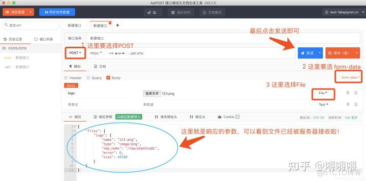
接口调试工具模拟Post上传文件——ApiPost
Learn more about materialapp and common attribute parsing in fluent

"Analysis of 43 cases of MATLAB neural network": Chapter 42 parallel operation and neural network - parallel neural network operation based on cpu/gpu
The 6th Blue Bridge Cup single chip microcomputer provincial competition

微信小程序中 在xwml 中使用外部引入的 js进行判断计算
《MATLAB 神经网络43个案例分析》:第42章 并行运算与神经网络——基于CPU/GPU的并行神经网络运算
2022-07-01:某公司年会上,大家要玩一食发奖金游戏,一共有n个员工, 每个员工都有建设积分和捣乱积分, 他们需要排成一队,在队伍最前面的一定是老板,老板也有建设积分和捣乱积分, 排好队后,所有

Jetpack's livedata extension mediatorlivedata
随机推荐
High performance and low power cortex-a53 core board | i.mx8m Mini
Oracle viewing locked tables and unlocking
树莓派GPIO引脚控制红绿灯与轰鸣器
2022-07-01:某公司年会上,大家要玩一食发奖金游戏,一共有n个员工, 每个员工都有建设积分和捣乱积分, 他们需要排成一队,在队伍最前面的一定是老板,老板也有建设积分和捣乱积分, 排好队后,所有
Interface debugging tool simulates post upload file - apipost
傅里叶级数
Which of PMP and software has the highest gold content?
Analyse de 43 cas de réseaux neuronaux MATLAB: Chapitre 42 opérations parallèles et réseaux neuronaux - - opérations parallèles de réseaux neuronaux basées sur CPU / GPU
[wireless image transmission] FPGA based simple wireless image transmission system Verilog development, matlab assisted verification
Recently, the weather has been extremely hot, so collect the weather data of Beijing, Shanghai, Guangzhou and Shenzhen last year, and make a visual map
5G时代全面到来,浅谈移动通信的前世今生
Suggestions on settlement solution of u standard contract position explosion
Kotlin 基础学习13
In wechat applet, the externally introduced JS is used in xwml for judgment and calculation
VS2010插件NuGet
Eight steps of agile development process
数据库文件逻辑结构形式指的是什么
h5中的页面显示隐藏执行事件
《MATLAB 神经网络43个案例分析》:第41章 定制神经网络的实现——神经网络的个性化建模与仿真
接口调试工具模拟Post上传文件——ApiPost