当前位置:网站首页>R language [logic control] [mathematical operation]
R language [logic control] [mathematical operation]
2022-07-07 05:43:00 【桜キャンドル yuan】
Catalog
3、 ... and 、 Mathematical operators
With e The exponential function at the bottom
Four 、 Matrix correlation operations
1. The inner product of a vector
2. The outer product of a vector
3. The transpose of the matrix
4. The addition and subtraction of matrices
5. The multiplication of a matrix
7. Operations related to the diagonal elements of a matrix
9. Eigenvalues and eigenvectors of matrices
10. Matrix Choleskey decompose
12. Extract the dimension of the matrix
13. Row sum of matrix 、 Column sum 、 Row average and column average
5、 ... and 、 Integral operations
6、 ... and 、 Negative number operation
7、 ... and 、 Mathematical functions
8、 ... and 、 Other utility functions
Apply functions to data frames and matrices
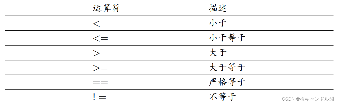
One 、 Logical operators
x <- c(3,0,-2,-5,7,2,-1)
y <- c(2,4,-1,0,5,1,-4)
x <= y
compare.xy <- (x<=y)
compare.xy 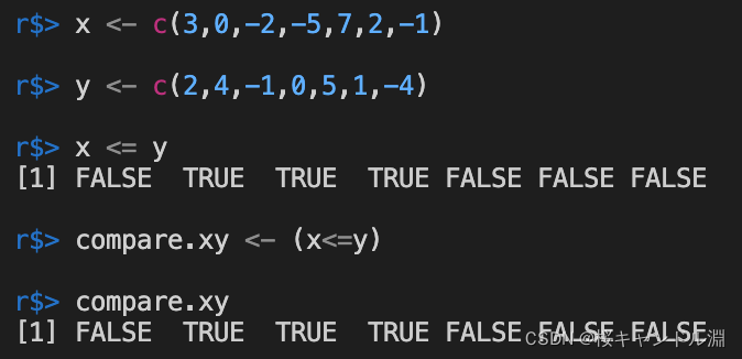
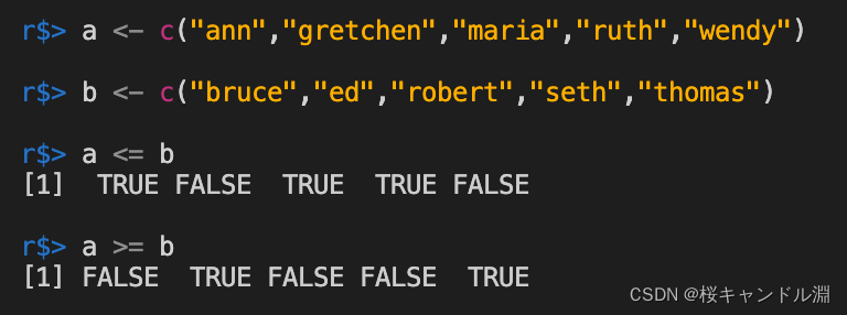
Strings are compared in character order
a <- c("ann","gretchen","maria","ruth","wendy")
b <- c("bruce","ed","robert","seth","thomas")
a <= b
a >= b
Two 、 Boolean operator
| Operator | describe |
| !x | Not x |
| x|y | x or y |
| x&y | x and y |
| isTRUE(x) | Judge x Is it true |
We can see from the following test code that if the element of the corresponding position meets the judgment of Boolean operator, it will return TRUE, If not, return to FALSE
x <- c(3,0,-2,-5,7,2,-1)
y <- c(2,4,-1,0,5,1,-4)
(x-y > -2)&(x-y < 2)
x[(x-y> -2)&(x-y < 2)]
(x-y >= -2)|(x-y <= 2)
x[(x-y>-2)&(x-y<2)]
(x-y > -2)
!(x-y > -2)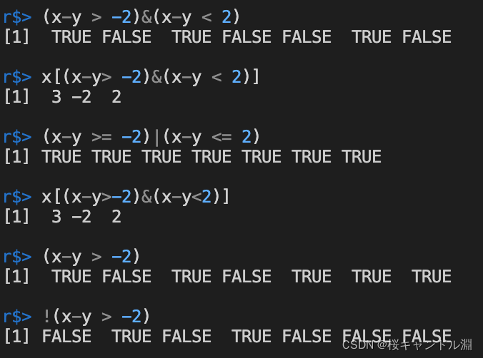
Index and related contents
x <- c(3,7,5,-2,0,-8)
x[3]
x[1:3]
x[c(2,4,5)]
x[1+3]
i =4
x[i]
x[-2]
x[-c(2,4,5)]
y <- c(2,7,-5,4,-1,6)
(x+y)[1:3]
z <- c("jan","feb","mar","apr","may","jun")
monthly.numbers <- data.frame(x,y,z)
monthly.numbers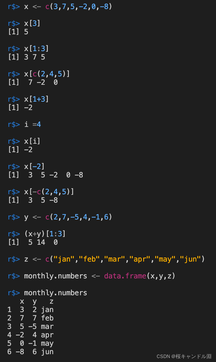
3、 ... and 、 Mathematical operators
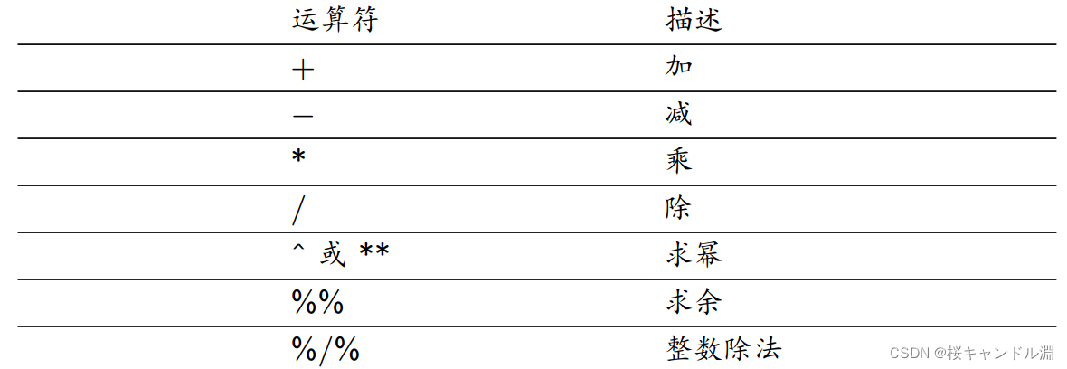
3+4 # 7
3-4 # -1
3*4 # 12
3/4 # 0.75
3^4 # 81
16**(1/4) # 2
13%%4 # 1
13%/%4 # 3
x <- c(-1,0,1)
exp(x)
y <- c(1,2,3,4)
sqrt(y) 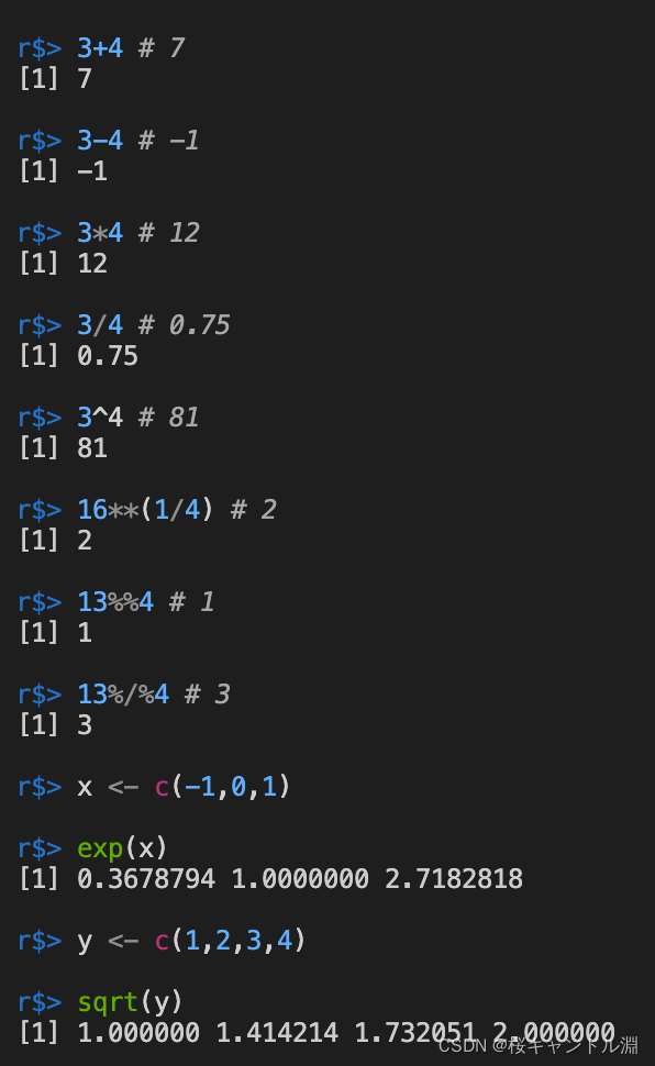
Quadratic function
xlow <- -1
xup <- 2
x <- xlow + (xup-xlow)*(0:100)/100
y <- x^2-x-1
plot(x,y,type="l")
y2 <- numeric(length(x))
# Draw a dot , Respectively by x,y2 The parameters of the corresponding position in the form of coordinate points , The type of line drawn is l, The straight line is a dotted line
#lty Parameters of can also be input 1,2,3 And other parameters to draw different styles of dimension lines
points(x,y2,type="l",lty="dashed")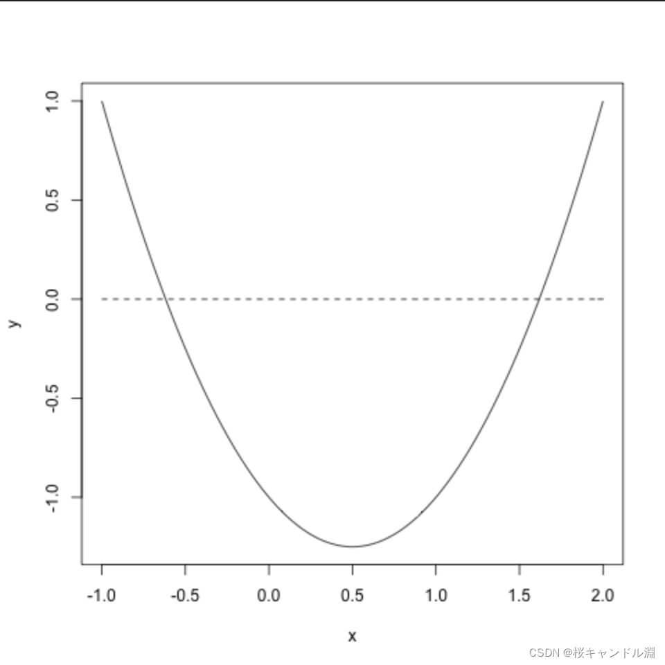
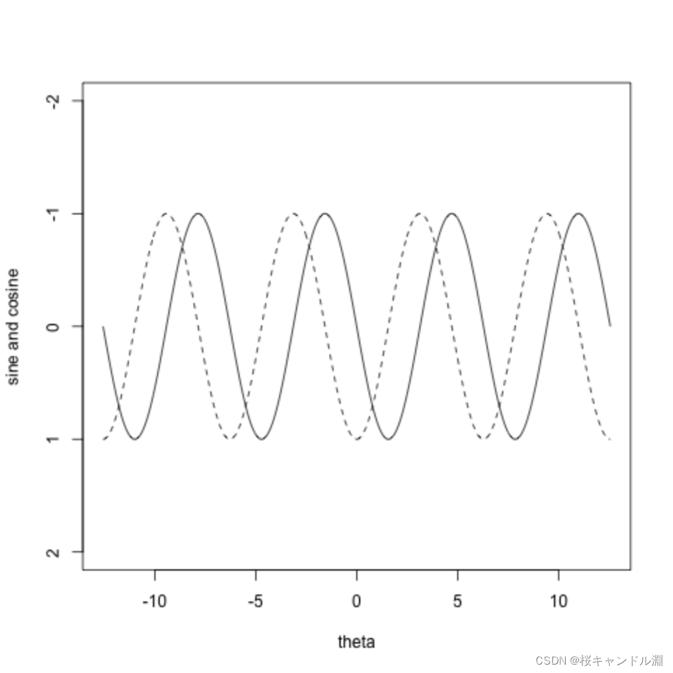
Trigonometric functions
# Set the upper and lower limits
th.low <- -4*pi
th.up <- 4*pi
theta <- th.low + (th.up-th.low)*(0:1000)/1000
y1 <- sin(theta)
y2 <- cos(theta)
plot(theta,y1,type="l",lty=1,ylim=c(2,-2),xlab="theta",
ylab="sine and cosine")
points(theta,y2,type="l",lty=2)
Polar coordinates
# Set the angle to 0-360 degree
theta <- 2*pi*(0:100)/100
r <- 1
x <- r*cos(theta)
y <- r*sin(theta)
# Set the size, length and width of our canvas to 4 Inch .
par(pin=c(4,4))
plot(x,y,type="l",lty=1)
With e The exponential function at the bottom
Use exp Function can be set to e Exponential function with base .
x <- 2
y <- exp(x)
z <- exp(0:10)
y
z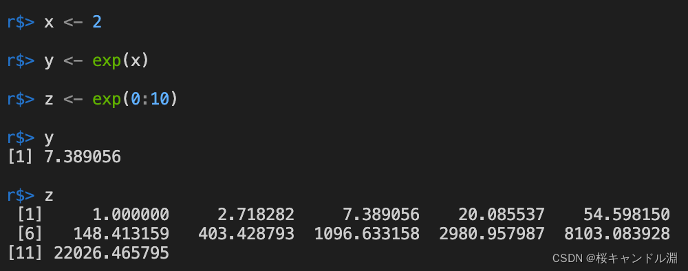
Logarithmic function
y = loga x, R Is represented by log(x,a)
y = ln x, R Is represented by log(x)
y = lg x, R Is represented by log10(x)
y = log2 x, R Is represented by log2(x)
If direct log(X) The default is e Bottom , That is to say ln(X)
w <- 0
log(w)
w <- 1:10
log(w)
w <- 10000
log10(w)
w <- 16
log2(w)
log(9,3)
log(64,8)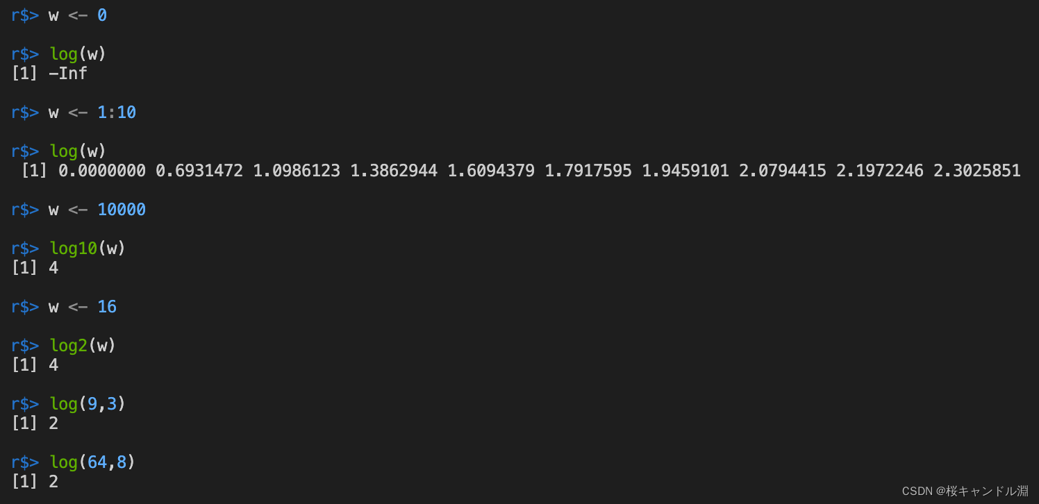
Four 、 Matrix correlation operations
1. The inner product of a vector
Use %*% perhaps crossprod Can generate the result of the inner product of vectors .
x <- 1:5
x
y <- 2*1:5
y
x %*% y
crossprod(x,y)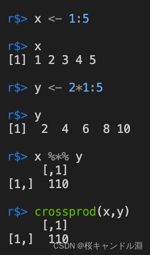
2. The outer product of a vector
Use %o% perhaps tcrossprod perhaps outer Can get the outer product of the vector , The outer product is the multiplication of elements in the same position
x %o% y
tcrossprod(x,y)
outer(x,y)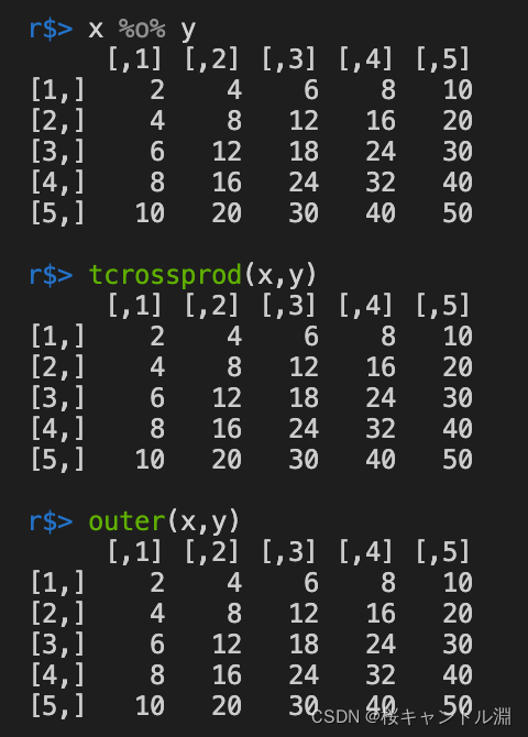
3. The transpose of the matrix
Use the transpose command t(x) We can realize the transpose of our matrix
x <- matrix(1:12,nrow=3)
x
y = matrix(1:12,ncol=3)
y
z = matrix(1:12,ncol=3, byrow=T)
z
X = t(x)
X
Y <- t(t(y))
Y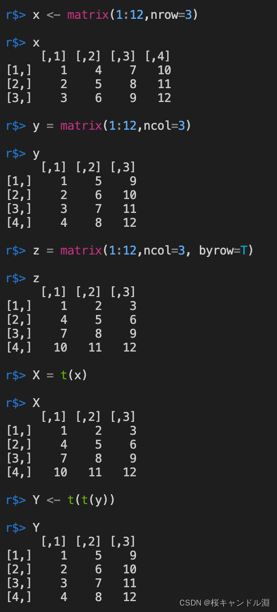
4. The addition and subtraction of matrices
x+t(z)
x-t(z)
x + 1
y <- 1:12
x + y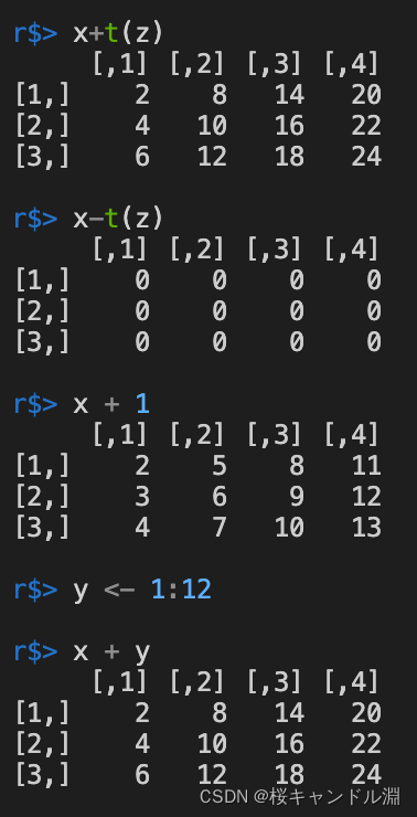
5. The multiplication of a matrix
Matrix multiplication will multiply every element in the matrix
a <- 3
M <- a*x
M
6. Matrix multiplication
Use %*% perhaps crossprod Can realize matrix multiplication
A = matrix(1:12,ncol=3)
B = matrix(1:18, nrow=3)
A
B
C = A%*%B
C
D = matrix(1:12, nrow=4, byrow=T)
D
t(A) %*% D 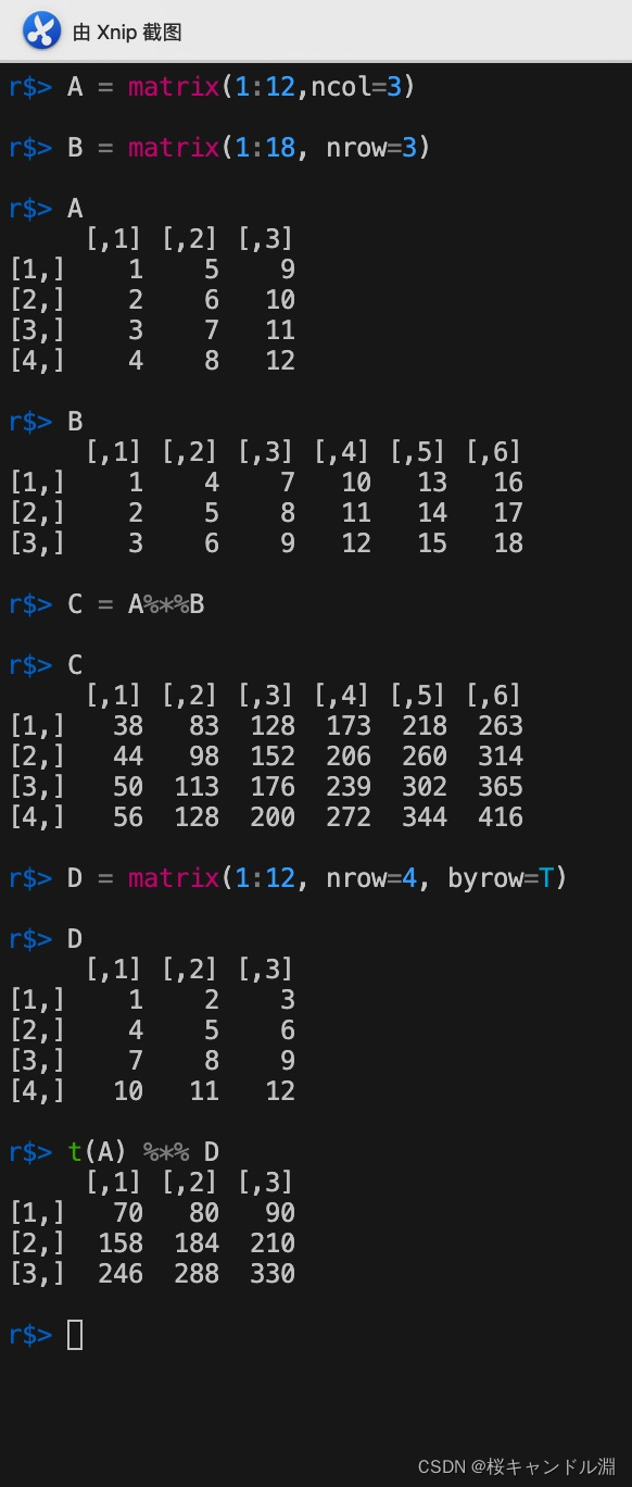
Used crossprod after , We don't need to transpose , It can also realize our A And D Multiplication of matrices . by comparison crossprod More efficient , in other words crossprod The matrix of the first parameter will be transposed and then multiplied by the matrix of the second parameter .
crossprod(A,D)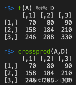
7. Operations related to the diagonal elements of a matrix
Use diag Function can get the elements on the diagonal of the current matrix , And splice it into a vector .
If diag If the parameter of is a vector , It will help us generate a diagonal matrix .
A = matrix(1:16,nrow=4)
A
diag(A)
diag(diag(A)) 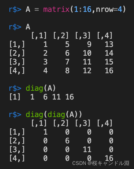
Generate a n The unit matrix of dimension
diag(n)
n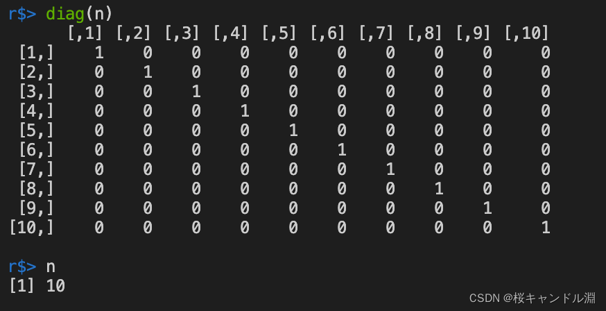
When diag When the parameter of is a vector , It will return a matrix with this vector as the main diagonal element .
x<-c(1,2,3,4,5)
diag(x) 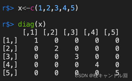
8. Matrix inversion
Use solve Function can find the inverse of our current matrix
AX=b,X=solve(A,b)
A = matrix(c(1,2,3,4,7,5,2,1,3,1,3,2,3,2,3,2),ncol=4)
A
solve(A)
b <- c(1,2,3,4)
# Calculation equations AX=b Solution
solve(A,b)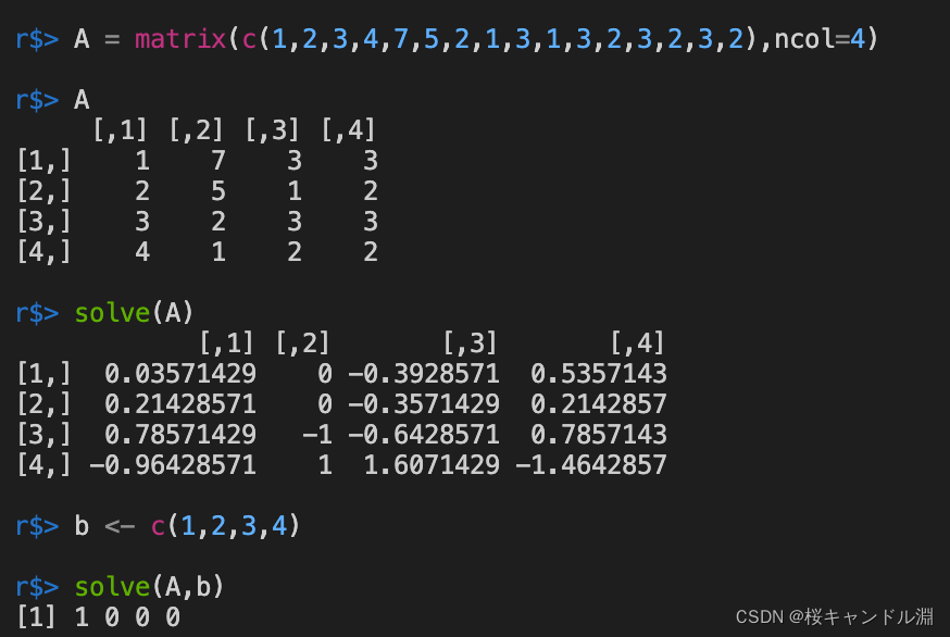
9. Eigenvalues and eigenvectors of matrices
Use eigen This method can calculate the eigenvalue of our current matrix and the corresponding eigenvector
values Represents the eigenvalue
vectors Represents the corresponding eigenvector
A = diag(4)+1
A
A.eigen = eigen(A,symmetric=T)
A.eigen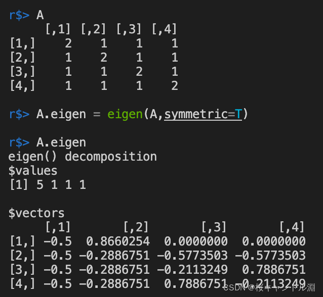
10. Matrix Choleskey decompose
Use our chol Method , It can realize the decomposition of our current matrix .
That is to say, Qiujiang A Decompose into P'P Of P Matrix
A = diag(4)+1
A
P <- chol(A)
P

11. Calculate determinant
Use det Function can calculate the determinant of our current matrix .
det(A)
12. Extract the dimension of the matrix
dim(A) Calculation of matrix A The number of rows and columns
ncol(A) Return matrix A Columns of
nrow(A) Return matrix A The number of rows
dim(A)
ncol(A)
nrow(A)
A
13. Row sum of matrix 、 Column sum 、 Row average and column average
A=matrix(1:16,ncol=4)
A
# Row sum
rowSums(A)
# Row average
rowMeans(A)
# Column sum
colSums(A)
# Column average
colMeans(A)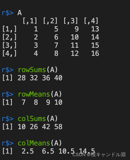
5、 ... and 、 Integral operations
integrate()
The first parameter is our formula for calculating the integral , The second parameter is our lower bound , The third parameter is our upper limit . In the following code Inf Infinity
integrand <- function(x) {1/((x+1)*sqrt(x))}
integrate(integrand, lower=0, upper=Inf)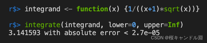
6、 ... and 、 Negative number operation
Generate complex vector .
complex(length.out,real=numeric(0),imaginary=numeric(0))
x <- 1+2i
y <- complex(1,1,1)
# Take the real part
Re(y)
# Take imaginary part
Im(y)
# Find module length
Mod(y)
# Find conjugate complex number
Conj(y)
# Judge whether it is plural
is.complex(y)
# Generate complex vector group
complex(re=1:4,im=2:3)
# Yes -2 Square root is not feasible
sqrt(-2)
# Yes -2+0i The square root is ok , Because this is a complex number operation
sqrt(-2+0i)
# If you want to be direct to -2 Find the square root , Or you could just say -2 Convert to plural form and open square root .
sqrt(as.complex(-2)) 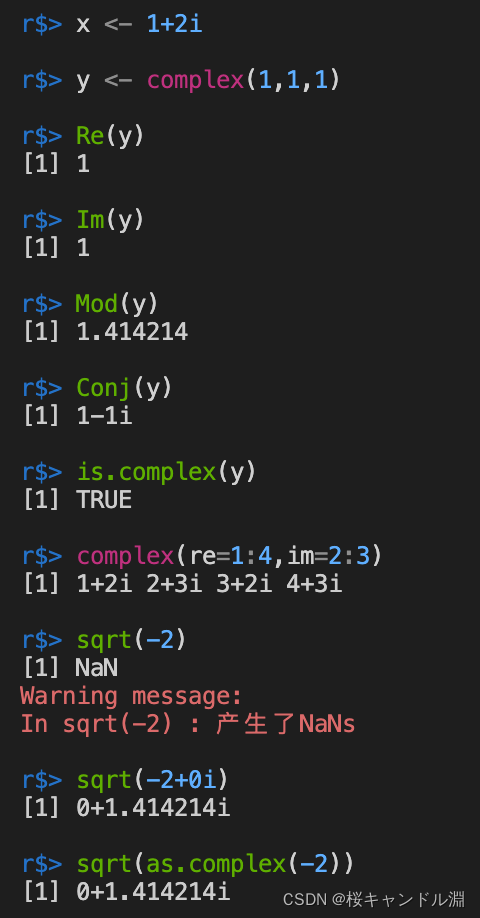
7、 ... and 、 Mathematical functions
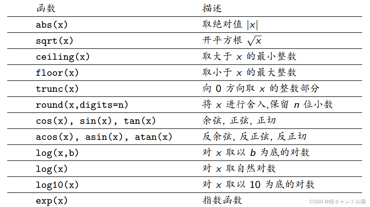
abs(-4.21) # 4.21
sqrt(16) # 4
ceiling(3.78) # 4
floor(3.78) # 3
floor(-3.78) # -4
trunc(-3.78) # -3
trunc(3.78) # 3
round(3.1415926, digits=4) # 3.1415
log(10,2) # 3.321928
log(10) # 2.302585
log10(10) # 1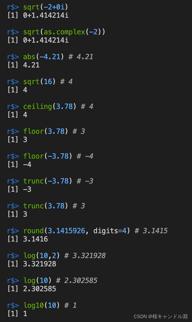
8、 ... and 、 Other utility functions
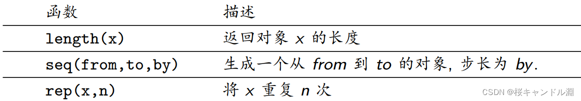
x<- c(1,2,3,4)
length(x)
rep(x,2)
rep(1,10)
seq(1,2,by=0.2) 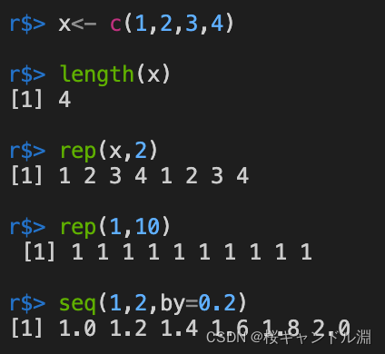
Apply functions to data frames and matrices
b <- c(1.23, 4.271, 9.2727)
# towards 0 Round the direction
trunc(b)
#runif(n, min, max) function , This function generates uniformly distributed values ,n Number of ,min and max Are the minimum and maximum values respectively , The default parameter is 0 and 1.
d <- matrix(runif(12),nrow=3)
# Take the logarithm of each element
log(d)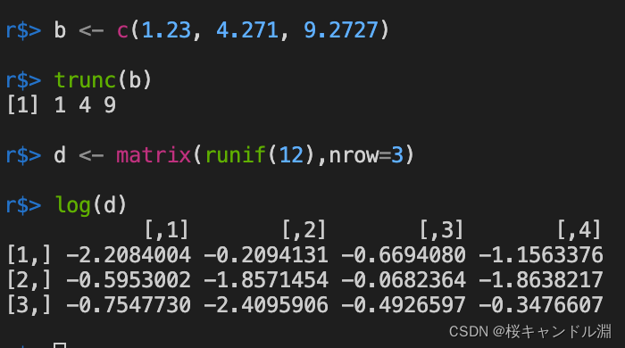
边栏推荐
- [binary tree] binary tree path finding
- ssm框架的简单案例
- JVM the truth you need to know
- R语言【逻辑控制】【数学运算】
- CVE-2021-3156 漏洞复现笔记
- [JS component] custom select
- Design, configuration and points for attention of network unicast (one server, multiple clients) simulation using OPNET
- 论文阅读【MM21 Pre-training for Video Understanding Challenge:Video Captioning with Pretraining Techniqu】
- 导航栏根据路由变换颜色
- Educational Codeforces Round 22 B. The Golden Age
猜你喜欢
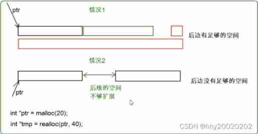
Dynamic memory management
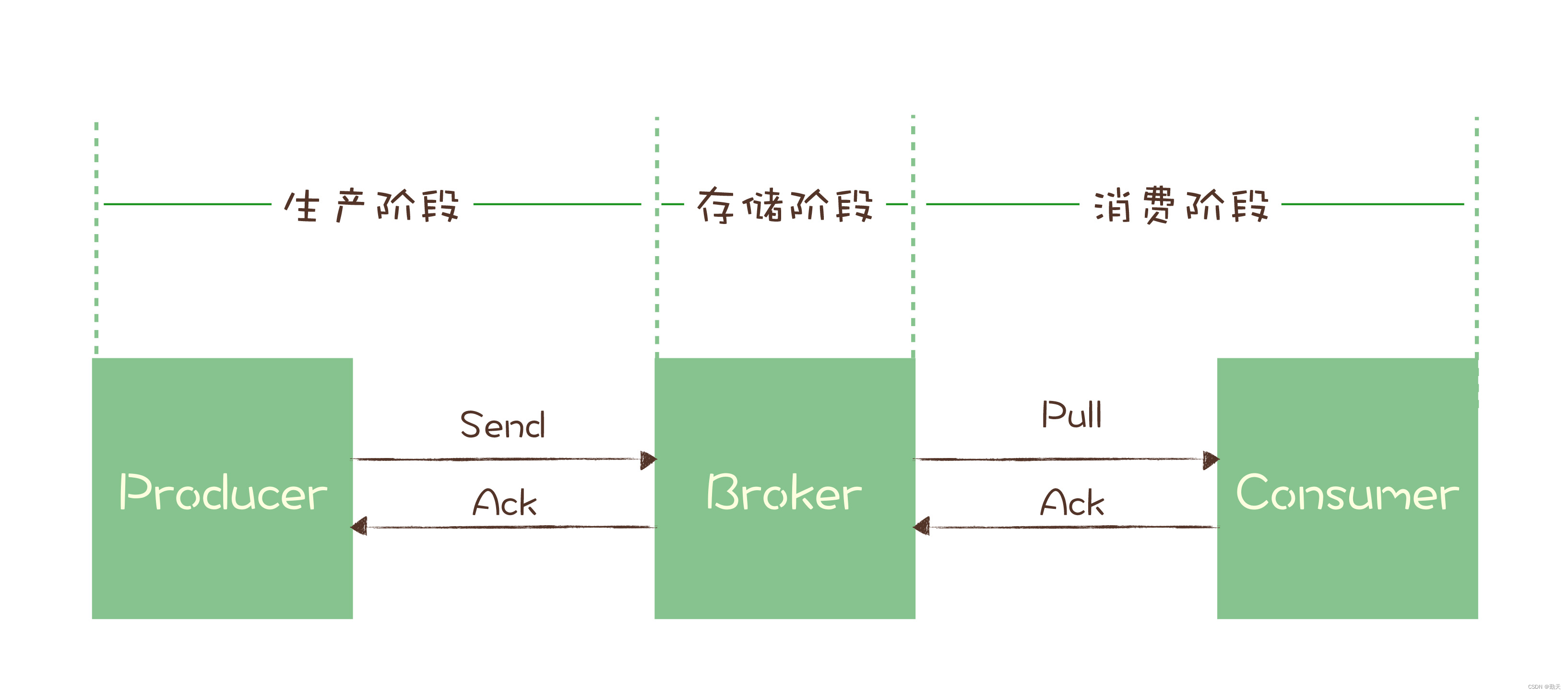
Message queuing: how to ensure that messages are not lost
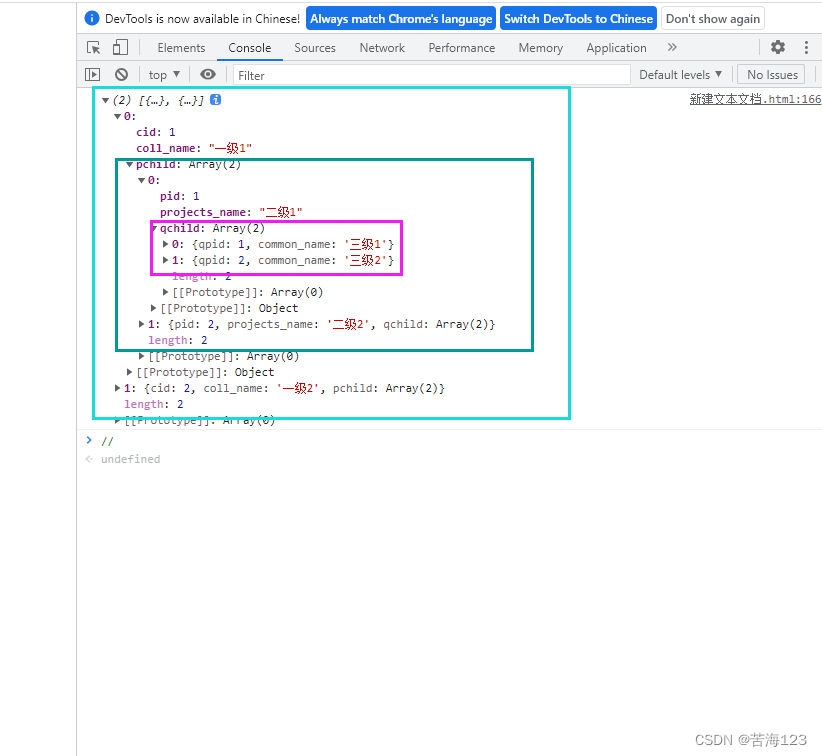
三级菜单数据实现,实现嵌套三级菜单数据
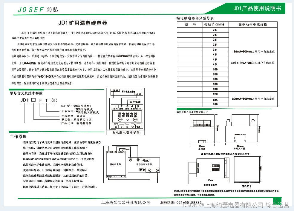
Leakage relay jd1-100
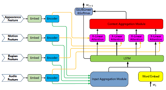
论文阅读【MM21 Pre-training for Video Understanding Challenge:Video Captioning with Pretraining Techniqu】
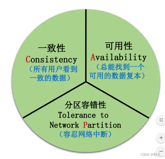
分布式事务介绍
AI人脸编辑让Lena微笑
![[JS component] date display.](/img/26/9bfc752c8c9a933a8e33b59e0488a2.jpg)
[JS component] date display.
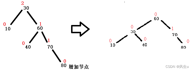
1. AVL tree: left-right rotation -bite
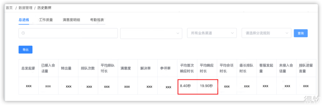
得物客服一站式工作台卡顿优化之路
随机推荐
Simple case of SSM framework
Initial experience of annotation
Jhok-zbg2 leakage relay
爬虫练习题(三)
Digital innovation driven guide
Flink SQL 实现读写redis,并动态生成Hset key
Egr-20uscm ground fault relay
Codeforces Round #416 (Div. 2) D. Vladik and Favorite Game
纪念下,我从CSDN搬家到博客园啦!
淘宝店铺发布API接口(新),淘宝oAuth2.0店铺商品API接口,淘宝商品发布API接口,淘宝商品上架API接口,一整套发布上架店铺接口对接分享
Codeforces Round #416 (Div. 2) D. Vladik and Favorite Game
ssm框架的简单案例
得物客服一站式工作台卡顿优化之路
拼多多商品详情接口、拼多多商品基本信息、拼多多商品属性接口
High voltage leakage relay bld-20
Pytorch builds neural network to predict temperature
pytorch_ 01 automatic derivation mechanism
When deleting a file, the prompt "the length of the source file name is greater than the length supported by the system" cannot be deleted. Solution
[paper reading] semi supervised left atrium segmentation with mutual consistency training
K6el-100 leakage relay