当前位置:网站首页>Isprs2021/ remote sensing image cloud detection: a geographic information driven method and a new large-scale remote sensing cloud / snow detection data set
Isprs2021/ remote sensing image cloud detection: a geographic information driven method and a new large-scale remote sensing cloud / snow detection data set
2022-07-07 13:03:00 【HheeFish】
ISPRS2021/ Cloud detection :A geographic information-driven method and a new large scale dataset for remote sensing cloud/snow detection A geographic information driven method and a new large-scale remote sensing cloud / Snow detection data set
Paper download
Open source code and data sets
0. Abstract
Geographic information such as altitude 、 Latitude and longitude are common but basic meta records in remote sensing image products . This article shows that , This set of records provides an important a priori for cloud and snow detection in remote sensing images . Intuition comes from some common geographical knowledge , Many of them are important , But it's often overlooked . for example , as everyone knows , Low latitude or low altitude areas are unlikely to have snow , Clouds in different geographical locations may have different visual appearances . Previous cloud and snow detection methods simply ignored the use of this information , But only based on image data ( Band reflectance ) To test . Because these priors are ignored , These methods are used in complex scenes ( many - Snow coexists ) It is difficult to obtain satisfactory performance . This paper presents a new neural network for cloud and snow detection —— Geographic information drives the network (GeoInfoNet). In addition to using image data , The model also integrates geographic information in the training and detection stages . Specially designed “ Geographic information encoder ”, The elevation of the image 、 Latitude and longitude are encoded into a set of auxiliary maps , Then input it into the detection network . The network can be trained end-to-end through intensive robust feature extraction and fusion . A new data set for cloud and snow detection is established “Levir_CS”, The dataset contains 4168 A gaofen-1 satellite image and corresponding geographical records , Larger than other data sets in this field 20 Many times . stay “Levir_CS” The experiment on shows that , The intersection rate of this method and cloud union is 90.74%, The intersection rate with snow is 78.26%. It has great advantages over other advanced cloud and snow detection methods . Feature visualization also shows , This method learns some important prior information close to common sense .
1. summary
In the last few decades , The rapid development of remote sensing technology helps people better understand the earth . Optical remote sensing technology is an important branch of remote sensing family , It has important application significance in target detection and other fields ( Zou Heshi ,2016; Lin et al ,2017a,b; Zou Heshi ,2017), Scene classification ( Shi et al ,2018) etc. . However , The imaging process of remote sensing images is often disturbed by clouds and snow . Previous literature shows , On average, clouds cover more than half of the earth's surface every day (Zhang and Xiao, 2014; Anheshi ,2015; Xie et al ,2017; Wu , stone ,2018). In some high latitudes , The ground may also be covered with ice and snow all year round . One side , The above two factors will greatly affect the processing and analysis of remote sensing images , Clouds can be a form of occlusion (Li et al., 2014, 2019b), Snow may dramatically increase reflectivity . On the other hand , Environmental research, such as climate research (Bi etc. ,2019) And ecological change analysis (Campbell etc. ,2005;Wang et al., 2018) Need cloud / Snow mask , But manually marking images is often time-consuming and expensive (Zhan et al., 2017). Automatic cloud and snow detection provides a way to generate pixel level clouds / Effective method of snow mask , Thus forming the basis of many remote sensing applications .
At an altitude of 、 longitude 、 Geographic information such as latitude is an important meta record in remote sensing image products . Such a set of records provides auxiliary and even vital information for image processing and analysis tasks . In the detection of clouds and snow , It also provides an important a priori . for example , as everyone knows , Low latitude or low altitude areas are unlikely to have snow , Clouds in different geographical locations may have different visual appearances . chart 1 Shows some sample images of clouds and snow . Each picture covers about 4 An area of... Million square kilometers , And there are different representatives in different positions on the earth . In recent years , Many deep learning cloud detection and snow detection methods have been proposed . Although great efforts and improvements have been made in this field , But the old method , Even the most advanced method , There are still limitations . One of the most serious defects of this method is that it ignores the use of geographic information in detection . in other words , The design of these deep learning methods is entirely based on image data ( Band reflectance ) Use , While ignoring other necessary priors , Such as height and position . In the complex scene where clouds and snow appear at the same time , These methods are often difficult to generate accurate cloud and snow masks .
This paper presents a new cloud and snow detection method based on deep learning . This method is called geographic information driven neural network (GeoInfoNet). Different from the previous focus on the use of image data ( Band reflectance ) The method of ignoring geographic information , This method designs a “ Geographic information encoder ”, The height of an image 、 Latitude and longitude are encoded into a set of two-dimensional maps . then , These maps are wisely integrated into the detection network , Then train the whole detection model in an end-to-end way . It can be seen that , With the integration of auxiliary information , The detection accuracy of clouds and snow is constantly improving . This method is superior to other advanced cloud and snow detection methods to a great extent . In addition to the new detection framework , A big data set for cloud and snow detection has also been established , The data set is composed of 4168 It is composed of images of gaofen-1 satellite , Of other data sets in the field 20 Many times . what's more , The dataset contains the corresponding geographic information , Including longitude 、 Latitude and high resolution elevation map of each image . The contributions of this paper are summarized as follows :
1) Different from the previous cloud and snow detection methods based on band reflectance , Directly ignore the geographical information of the image , A new deep learning framework is proposed “GeoInfoNet”, Integrate geographic information into the detection process , Automatic learning a priori detection . The encoder will provide auxiliary information such as altitude 、 Longitude and latitude are encoded as a group 2D Map , The detection network can effectively learn pixels in an end-to-end manner .
2) Extensive research on feature visualization shows what a priori knowledge the framework learns , And the contribution of different parts to the test results .
3) A new data set is established for cloud and snow detection , This dataset is larger than the previous dataset 20 times . what's more , The geographic information of each image is recorded in the data set , This information is not included in previous data sets .
The following contents of this article are organized as follows . The second section introduces the related work of this method . The first 3 Section describes the proposed method in detail . In the 4 In the festival , The data set is given Levir_CS Details of . In the 5 In the festival , Extensive experiments have been carried out on this method , And in the first place 6 Section presents a discussion . Last , The seventh part summarizes this paper .
2. Method
This section describes the test method in detail , And how to encode and integrate geographic information into the network
2.1.GeoInfoNet summary
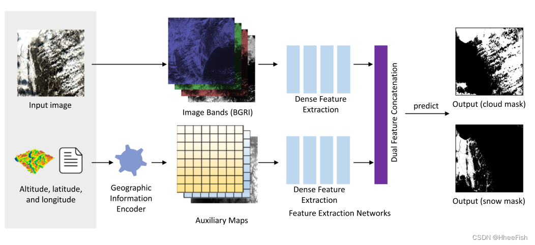
chart 2. Overview of the proposed approach . Put forward a kind called GeoInfoNet The new network , The network uses image data and auxiliary geographic information to detect cloud and snow . The geographic information encoder aims to encode this information into a set of auxiliary maps . These two network branches are characterized by “ Feature extraction network ” Extracted , These include “ Dense feature extraction ” Module and “ Double feature stitching ” modular . The previous module can extract the representative features of each branch , The latter module is used to generate fine feature representation , Further used to generate cloud and snow masks
chart 2 Shows an overview of the method . The proposed geographic information network is an end-to-end network , Using input images and a set of auxiliary maps . The auxiliary map is composed of Geographic information encoder Generate , In the fourth 2.2 Described in the section . stay GeoInfoNet in , follow DenseNet(Huang wait forsomeone ,2017) As the backbone network , Extract multi-scale dense features from the input image and auxiliary map respectively . then , These features extracted from these two branches will be merged and used to generate the final cloud and snow mask . Two basic modules in this method , Composition “ Feature extraction network ” Of “ Dense feature extraction ” and “ Double feature series ”, In the fourth 2.3.1 Section and section 2.3.2 Section .
2.2. Geographic information encoder Geographic information encoder
The geographic information encoder is designed to integrate three types of meta records ( namely longitude 、 Latitude and altitude ) And image coding into a set of auxiliary maps . This module can be considered as the proposed geographic information network GeoInfoNet Preprocessing module . These generated maps have the same space size as the input image , But there may be a different number of channels . chart 3 Shows the processing pipeline of the geographic information encoder .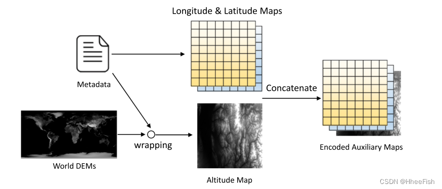
chart 3. Processing pipeline of geographic information encoder . For input images , Based on the equation (1) Generate longitude and latitude maps from metadata ALat. Input the height map of the image AAlt Also through the world DEM It is generated by wrapping it into image projection coordinates in pixel mode . Last , Connect these three mappings to generate the final encoded . Auxiliary map .
Give a picture of h×w Size remote sensing image , First, record the longitude and latitude in the upper left corner and the lower right corner . then , Through affine transformation model, longitude map and latitude map are generated ALat(Warmerdam,2008;Zhao wait forsomeone ,2010). about y A pixel in the row (0⩽y<h) and x Column (0⩽x<w), Along the ALong(y,x) The corresponding longitude and latitude ALat(y,x) It can be calculated as follows :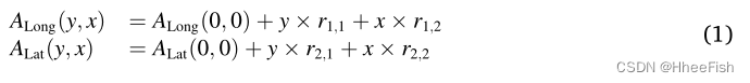
among , Along the ALong(0,0) and ALat(0,0) Is the longitude and latitude value of the upper left corner of the image .r1,1、r1,2、r2,1 and r2,2 yes x and y Longitude in direction / Latitude resolution unit , It can be obtained from the metafile of image products , It can also be estimated from the coordinates of the four image corners and center points .
In addition to longitude and latitude , The height of the image is also encoded into another auxiliary map AAlt in . Given an image and its corresponding longitude / Latitude information , The global digital elevation model can be (DEM) Wrap the projection coordinates of this image to generate an elevation map AAlt. For most optical remote sensing image products , Image height information is not included in the metafile . In this paper , The use of DEM Is based on 2000 Space Shuttle Radar terrain mission (SRTM) Created by the collected data , A resolution of 3 Arcseconds ( Spatial resolution :90 rice ).
The final encoded auxiliary mapping of each input image A It can be expressed as the concatenation of the above three mappings in the channel dimension , As shown below ,
among ,A The dimension of is (h,w,3).
2.3. Feature extraction network
2.3.1. Dense feature extraction
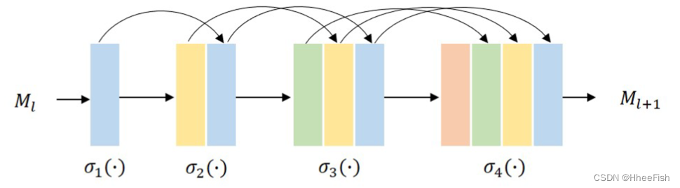
chart 4.4 Diagram of layer dense block . Each convolution layer takes all the previous feature maps as input .
In the cloud and snow detection method based on deep learning , Learning robust feature representation is very important for detection tasks . Because improving the network backbone is not the focus of this article , Therefore, a simple method called “DenseNet”(Huang wait forsomeone ,2017) The famous trunk of , It can achieve the most advanced results in various tasks , As a backbone network for extracting high-quality features from the input data array .
DenseNet It is composed of multiple dense blocks . In each piece , Features from all previous convolutions are connected . Formally , The first (l+1) Layer feature mapping Ml+1 It can be calculated as follows ,
among σ(⋅) Represent nonlinear transformations on features . chart 4 Shows Ml+1 Calculation process .
According to the equation 3, In the calculation Ml+1 Preserve feature mapping in the process of M1、M2、…、Ml. Considering that the concatenation of feature maps requires space , Compared with the number of filters in the standard convolution network , Number of filters per convolution u Set to a smaller number , for example ,u=32, for example VGG(Simonyan and Zisserman,2015) and ResNets(He wait forsomeone ,2016). under these circumstances ,(l+1) The number of input feature maps in the layer will be u1+32×l, among u1 Is the number of characteristic graphs in the first layer ,32 Is the filter in each layer , You could say yes growth rate . A small growth rate not only adjusts the number of features , This makes the feature extraction network become relatively deep , It also balances the number of features added in each layer , Because the newly added information should be considered equally important .
Nonlinear transformation σ(⋅) In the network , There are two types of operations , Normalization operation ( Batch normalization (Ioffe and Szegedy,2015)) And nonlinear activation operation ( Correct linear unit function (Glorot wait forsomeone ,2011)). It should be noted that ,1×1 Convolution can be placed in 3×3 Before convolution , This seems to be a “ bottleneck ”, What kind of person (2016)、 Huang et al (2017) in , These settings can improve computing efficiency . therefore , follow “ Bottleneck design ” Thought ,σ(⋅) With BN-ReLU-Conv(1×1)-BN-ReLU-Conv(3×3) Formal design of , Each of them Conv(1×1) Output 4u Feature mapping .
In addition to the above dense connection modules , Some are also designed in the network Down sampling module , In order to reduce the size of the feature map in space and improve the computational efficiency (Wu and Shi,2018). These modules follow BN-ReLU-Conv(1×1)-Pool( Average 2×2) The configuration of is designed as a transition block , And placed between dense blocks . there 1×1 Convolution output Half of the input feature mapping .
Huang et al (2017) Several different types of DenseNet To configure , Include DenseNet121、DenseNet169、DenseNet201 and DenseNet264.“DenseNetX” Number in “X” Indicates the number of convolution layers used in the classification network . In the dense feature extraction module , Considering the computational efficiency and GPU Balance of memory cost , Adopted DenseNet169 Configuration of . The module receives the input array , The array first passes through the initial convolution layer (“Conv_0”) And the initial pool layer (“Pool_ 0”) To deal with , Then, four dense blocks and three transition blocks are passed accordingly . And Huang wait forsomeone (2017) The settings in are different ,“Conv_0” The step size of is set to 1, And deleted the cloud and snow detection task The last classification layer . The configuration details of the dense feature extraction module are shown in the table 1 Shown .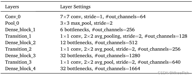
surface 1 Configuration of dense feature extraction module .
2.3.2. Double feature series
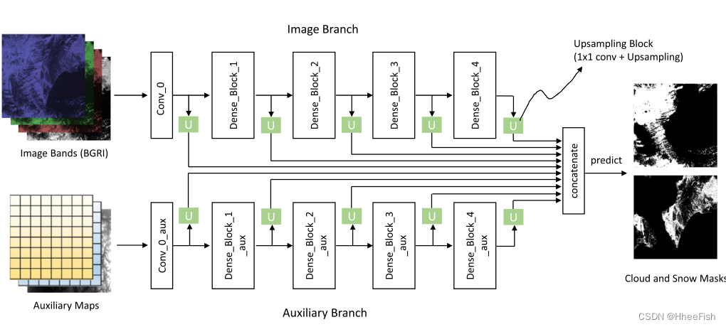
chart 5. Details of dense feature extraction module . This method receives two types of input at the same time , That is, input the original remote sensing image RGBI Band and auxiliary map encoded by geographic information encoder . In both branches , The dense features are all composed of “convo_0” Layer and the following four dense blocks are extracted . Sample the features of different blocks to the same size , And pass 1×1 Convolution adjusts the number of channels , Then connect all these features along the channel dimension . Last , Use the prediction layer to generate pixel level fractional images of clouds and snow .
In the above feature extraction process , As the layer deepens , The number of output characteristic graphs becomes larger . Compared with the input spatial resolution , Final output The spatial resolution is reduced to 16× sampling , As shown in the table 1 Shown . To generate a high-resolution cloud and snow mask , Feature resolution must be improved by extracting features . This can be achieved by merging the features of different blocks and generating fine-grained feature representations . therefore , The dense feature cascade module is designed for this purpose . In this module , Blue green red infrared (BGRI) Input the initial features of the image and coding auxiliary map .
Pictured 5 Shown , For network ( Input image branch and auxiliary map Branch ), Firstly, bilinear interpolation is used to sample the spatial features of each feature block up to the size of the input image . then , Connect the upsampling features along the channel dimension . Before cascading , We also use 1x1 Convolution to adjust the channel dimension of each block feature , So that they have the same number of channels . The intuition behind this operation is , Suppose for all blocks in the network , Features should be viewed with the same importance in cloud and snow detection tasks . The final join feature of all blocks from both branches M It can be expressed as :
among , Subscript “img” and “aux” Respectively from BGRI Characteristics of image branch and auxiliary information branch . Subscript “0–4” Representing the dense feature extraction module “Conv_ 0”、“Dense_ block_ 1”、“Dense_ block_ 2”、“Dense_ block_ 3” and “Dense_ block_ 4” Upsampling feature in .
2.3.3. Loss setting
In the proposed geographic information network , Use prediction layer ( belt 1×1 Convolution layer of filter ) Generate pixel level fractional graphs of different categories : background S1、 cloud S2 And snow S3. Use softmax Function normalizes the output fractional graph , And convert the pixel fraction (−∞,∞) To probability [0,1]. Each class t={1,2,3} The probability graph of Pt It can be expressed as :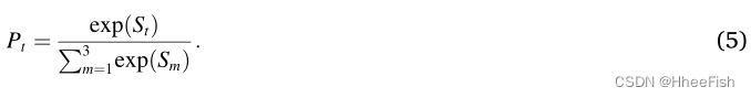
Because cloud and snow detection is essentially a pixel level classification process , Therefore, by using standard pixel level classification loss ( Also known as cross entropy loss ) To train the Internet . hypothesis ym∈ {0,1} Express m Ground truth label of class . The loss function of each pixel is expressed as follows :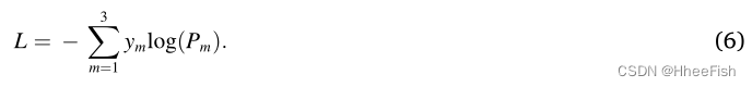
Last , Calculate the average loss of all pixels of all images in the training set as the final loss function .
3.Levir_CS: A new large-scale cloud and snow detection data set
Established a system called “Levir_CS” Large scale data sets of , among “C” Respectively means cloud ,“S” Respectively means snow . Because the name of the author's laboratory is “ Study 、 Vision and Remote Sensing Laboratory ”, And ( Zou Heshi ,2017) similar , The name of the dataset is in “Levir” start . Although some public datasets on this topic have been published in the past , But they are relatively small , Does not contain geographic information . Besides , There is no public data set for snow detection before . surface 2 It shows the comparison between our data set and other public cloud detection data sets (Scaramuzza wait forsomeone ,2011;Foga wait forsomeone ,2017;Li wait forsomeone ,2017). And watch 2 Compared to other datasets listed in ,LEVIR_CS The number of scenes in is larger than other data sets 20× above , therefore , The proposed data set is called “ On a large scale ”. The proposed Levir_CS Datasets in https://github.com/permanentCH5/GeoInfoNet
Gaofen-1 satellite (GF-1) In the sun synchronous orbit , The angle is 98.0506◦ The average orbital height is 645 km . The return visit time is 4 God . The descending node is in the morning 10:30.GF-1 Wide field sensor (GF-1 WFV) The radiation resolution is 10 position . One GF-1 WFV scene , Each scene is wide 211 km , Long 192 km , Instantaneous field of view in all four bands (IFOV) by 16 rice ×16 rice . The spectral range is 450 nm to 890 nm. To be specific , The spectral ranges of these bands are 450–520 nm( Blue band or band 1)、520–590 nm( Green band or band 2)、630–690 nm( Red band or band 3)、770–890 nm( Near infrared band or band 4).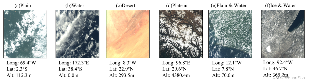
chart 7. Proposed Levir_CS Some example scenarios with different types of ground features in the dataset . At the top of each scene , The types of ground features are given . At the bottom of each scene , It shows the longitude and latitude of the center point and the average height of the image .
What we proposed Levir_CS It's made up of 4168 individual GF-1WFV Scene composition . These scenes were randomly divided into two groups , A group contains 3068 A training set of scenes and a set containing 1100 A test set of scenarios . The scenes in the dataset have global distribution , Pictured 6 Shown . They cover different types of ground features , Like a plain 、 plateau 、 water 、 The desert 、 Ice, etc . There are also combinations of the above ground feature types . chart 7 Some sample scenarios are shown . Besides , Because these scenes are globally distributed , therefore , These scenes may contain different types of climatic conditions , For example, desert climate ( See the picture 7(c)) Or ocean climate ( See the picture 7(b,e)), This may help something like (Bi wait forsomeone ,2019) Related research . All scenes are in 2013 year 5 Month to 2019 year 2 Monthly collection , Download from http://www.cresda.com/.
In the proposed LEVIR_CS Data set , For each scene , Used After the radiation calibration process 1A Level product data , And the current data Without systematic geometric correction . This is because in many practical cases , Cloud and snow detection needs to be performed at this product level , To save geometric correction time or browse quickly . Data set users can provide rational polynomial coefficients (RPC) Documents obtained ac, In order to carry out the geometric correction of the system when necessary . Besides , In order to reduce the processing time of each scene and accelerate the learning process of global information , Be similar to (Zou wait forsomeone ,2019),LEVIR_CS The images in the dataset are 10 Downsampling . about LEVIR_CS Every scenario in the dataset , The image size is 1320×1200, The spatial resolution is 160m. all Four bands Both use . therefore ,DEM(90 m) The resolution of is high enough in height map generation . therefore , choice SRTM Data as DEM Source .
In the proposed LEVIR_CS Data set , For each scene , provide Geo referenced multispectral images 、 Digital elevation model image And corresponding Ground live image . The map projection system used in the data set is World geodetic system (WGS), Using the latest version (WGS 84). Through the map projection system , All images of each scene can be registered through geographic information . therefore , Climatic conditions have nothing to do with the generation of geo referenced images . For generating digital elevation model images , The average generation time of each scene is 45.62 second .
For all images in the dataset , Their pixel level tag masks are manually marked into three categories :“ background ”( Marked as 0)、“ cloud ”( Marked as 127) and “ snow ”( Marked as 255). And ( Li et al ,2017 year ) similar , The marking process is in Adobe Photoshop Finish in . Blue of the original image 、 The green and red bands are combined into RGB Images , For manual marking . In order to improve the efficiency of tagging , And (Lu wait forsomeone ,2019) similar , First, perform pre segmentation by manually setting the threshold , Such as traditional physical methods (Zhong wait forsomeone ,2017) Shown . then , These pre segmented regions are classified into coarse pixels . The boundaries of cloud or snow areas are usually blurred . Compared with previous studies ( Li et al ,2017 year 、2019a) equally , Use the brush tool ( Less than 10 Pixels ) Or the lasso tool carefully marks these areas of the image . For thin cloud areas , If the ground cover is not visible , Then mark it as cloud . For shaded areas , Because it is very dark and the area is not visible , So mark it as the background . When marking difficult areas , Use the magnifying glass tool ( The local area is enlarged by more than 200%), This helps the marker identify the exact category of pixels . Cloud shadow detection is not the focus of this article , therefore , This class is not marked .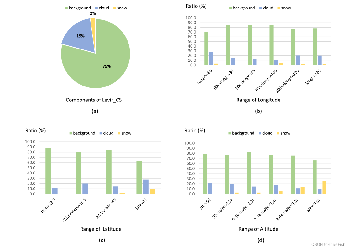
chart 8.Levir_CS The statistics of the dataset come from different views .(a) The number of pixels in the three categories : The background accounts for the most (79.2%), And snow accounts for the least (2.2%). Cloud pixels account for 18.6%.(b) -(d) From longitude 、 Latitude and altitude view marker components . It can be seen that , The distribution of these three categories in different regions is very different .
chart 8 Shows Levir_CS Statistics of the dataset . Calculate the distribution of label components from different views . Pictured 8(a) Shown , stay Levir_CS in , Background pixels account for the most (79.2%), And snow accounts for the least (2.2%). Cloud pixels account for 18.6%. chart 8(b)-(d) Longitude is displayed respectively 、 Label components in latitude and altitude view . The following observations can be summarized from these figures :
- In different places , The total of these three types of pixels is very different
- Clouds are common in different geographical locations . for example , In North America , Clouds appear in different kinds and forms (Sun wait forsomeone ,2017 year )
- From the perspective of longitude , It can be seen that , stay Snow is less likely in the following ranges :−60◦⩽ Long ⩽30◦ ( The Atlantic ocean )( See chart 7(c,e) Example ), And in the 65◦⩽ Long ⩽100◦, It's easier to find snow ( An example is shown in 7(d)) From the perspective of latitude , It can be seen that most of the snow occurs at high latitudes (lat)⩾43◦) ( An example is shown in 7(f)).
- according to (Tran wait forsomeone ,2019 year ) The data of , In the U.S. , The number of snow days in high latitudes is higher . Besides , In polar high latitudes , Ice and snow will not melt in some seasons (Selkowitz and Forster,2016). There is almost no snow in the equatorial region (−23.5◦⩽ Latin America ⩽23.5◦)( An example is shown in 7(a、c、e).
- from Altitude Look at , It can be seen that , At an altitude below 500 It's an area of about 200 meters , The percentage of cloud cover is relatively high ( For example, see Figure 7(a、b、e)), The percentage of snow increases gradually with the increase of altitude ( For example, see Figure 7(d、f)). Usually , High altitude areas are mountainous areas , The snow here changes regularly with the season ( Wang et al ,2018). For altitude 3400 Areas more than meters , It's easier to find snow than clouds ( An example is shown in 7(d)).
From the above statistics, we can see that , Using geographic information to detect cloud and snow is of great significance .
边栏推荐
- Aosikang biological sprint scientific innovation board of Hillhouse Investment: annual revenue of 450million yuan, lost cooperation with kangxinuo
- Talk about four cluster schemes of redis cache, and their advantages and disadvantages
- 处理链中断后如何继续/子链出错removed from scheduling
- Per capita Swiss number series, Swiss number 4 generation JS reverse analysis
- .Net下极限生产力之efcore分表分库全自动化迁移CodeFirst
- Analysis of DHCP dynamic host setting protocol
- . Net ultimate productivity of efcore sub table sub database fully automated migration codefirst
- 在字符串中查找id值MySQL
- ip2long与long2IP 分析
- Leetcode skimming: binary tree 20 (search in binary search tree)
猜你喜欢
Differences between MySQL storage engine MyISAM and InnoDB
聊聊Redis缓存4种集群方案、及优缺点对比
How to continue after handling chain interruption / sub chain error removed from scheduling
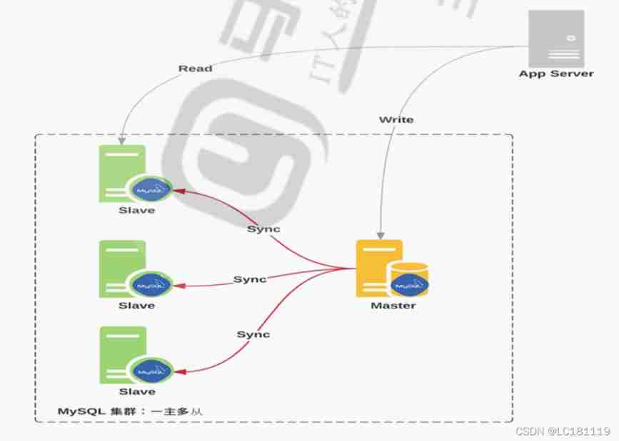
MySQL master-slave replication

Sequoia China completed the new phase of $9billion fund raising

ICLR 2022 | pre training language model based on anti self attention mechanism
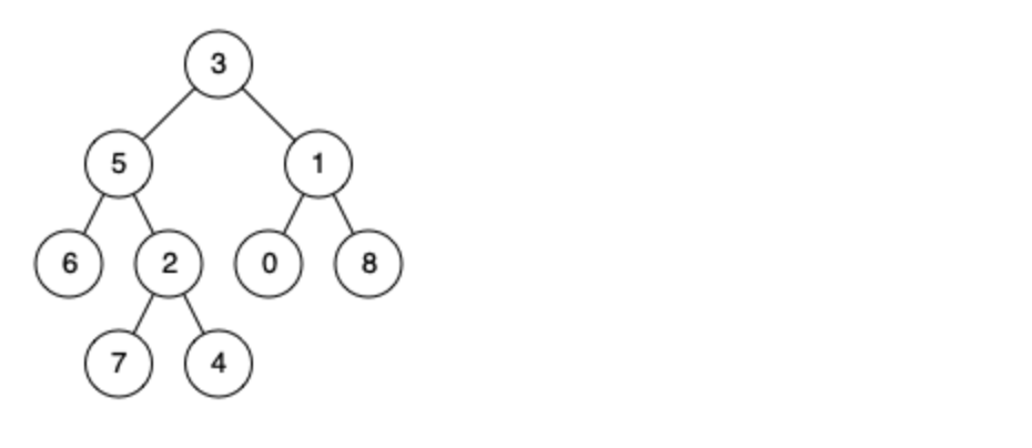
Leetcode brush question: binary tree 24 (the nearest common ancestor of binary tree)

Sample chapter of "uncover the secrets of asp.net core 6 framework" [200 pages /5 chapters]
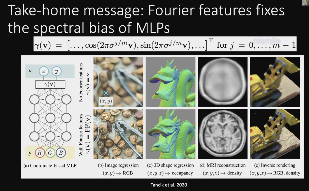
基于NeRF的三维内容生成
Smart cloud health listed: with a market value of HK $15billion, SIG Jingwei and Jingxin fund are shareholders
随机推荐
[binary tree] delete points to form a forest
.Net下極限生產力之efcore分錶分庫全自動化遷移CodeFirst
【无标题】
MySQL importing SQL files and common commands
[learn microservices from 0] [03] explore the microservice architecture
How to reset Google browser? Google Chrome restore default settings?
xshell评估期已过怎么办
共创软硬件协同生态:Graphcore IPU与百度飞桨的“联合提交”亮相MLPerf
Practical example of propeller easydl: automatic scratch recognition of industrial parts
Grep of three swordsmen in text processing
File operation command
- Oui. Migration entièrement automatisée de la Sous - base de données des tableaux d'effets sous net
日本政企员工喝醉丢失46万信息U盘,公开道歉又透露密码规则
MySQL master-slave replication
[learn wechat from 0] [00] Course Overview
HZOJ #235. Recursive implementation of exponential enumeration
云检测2020:用于高分辨率遥感图像中云检测的自注意力生成对抗网络Self-Attentive Generative Adversarial Network for Cloud Detection
About the problem of APP flash back after appium starts the app - (solved)
聊聊Redis缓存4种集群方案、及优缺点对比
How to reset Firefox browser