当前位置:网站首页>[optimtool.unconstrained] unconstrained optimization toolbox
[optimtool.unconstrained] unconstrained optimization toolbox
2022-07-04 21:41:00 【DeeGLMath】
【optimtool.unconstrain】 Unconstrained optimization toolbox
# import packages
%matplotlib inline
import sympy as sp
import matplotlib.pyplot as plt
import optimtool as oo
def train(funcs, args, x_0):
    f_list = []
    title = ["gradient_descent_barzilar_borwein", "newton_CG", "newton_quasi_L_BFGS", "trust_region_steihaug_CG"]
    colorlist = ["maroon", "teal", "slateblue", "orange"]
    _, _, f = oo.unconstrain.gradient_descent.barzilar_borwein(funcs, args, x_0, False, True)
    f_list.append(f)
    _, _, f = oo.unconstrain.newton.CG(funcs, args, x_0, False, True)
    f_list.append(f)
    _, _, f = oo.unconstrain.newton_quasi.L_BFGS(funcs, args, x_0, False, True)
    f_list.append(f)
    _, _, f = oo.unconstrain.trust_region.steihaug_CG(funcs, args, x_0, False, True)
    f_list.append(f)
    return colorlist, f_list, title
#  Visualization functions : Parameter transmission interface ( Color list , Function value list , Title list )
def test(colorlist, f_list, title):
    handle = []
    for j, z in zip(colorlist, f_list):
        ln, = plt.plot([i for i in range(len(z))], z, c=j, marker='o', linestyle='dashed')
        handle.append(ln)
    plt.xlabel("$Iteration \ times \ (k)$")
    plt.ylabel("$Objective \ function \ value: \ f(x_k)$")
    plt.legend(handle, title)
    plt.title("Performance Comparison")
    return None
Extended Freudenstein & Roth function
f ( x ) = ∑ i = 1 n / 2 ( − 13 + x 2 i − 1 + ( ( 5 − x 2 i ) x 2 i − 2 ) x 2 i ) 2 + ( − 29 + x 2 i − 1 + ( ( x 2 i + 1 ) x 2 i − 14 ) x 2 i ) 2 , x 0 = [ 0.5 , − 2 , 0.5 , − 2 , . . . , 0.5 , − 2 ] . f(x)=\sum_{i=1}^{n/2}(-13+x_{2i-1}+((5-x_{2i})x_{2i}-2)x_{2i})^2+(-29+x_{2i-1}+((x_{2i}+1)x_{2i}-14)x_{2i})^2, x_0=[0.5, -2, 0.5, -2, ..., 0.5, -2]. f(x)=i=1∑n/2(−13+x2i−1+((5−x2i)x2i−2)x2i)2+(−29+x2i−1+((x2i+1)x2i−14)x2i)2,x0=[0.5,−2,0.5,−2,...,0.5,−2].
# make data(4 dimension)
x = sp.symbols("x1:5")
f = (-13 + x[0] + ((5 - x[1])*x[1] - 2)*x[1])**2 + \
    (-29 + x[0] + ((x[1] + 1)*x[1] - 14)*x[1])**2 + \
    (-13 + x[2] + ((5 - x[3])*x[3] - 2)*x[3])**2 + \
    (-29 + x[2] + ((x[3] + 1)*x[3] - 14)*x[3])**2
x_0 = (1, -1, 1, -1) # Random given
# train
color, values, title = train(funcs=f, args=x, x_0=x_0)
# test
test(color, values, title)

Extended Trigonometric function:
f ( x ) = ∑ i = 1 n ( ( n − ∑ j = 1 n cos x j ) + i ( 1 − cos x i ) − sin x i ) 2 , x 0 = [ 0.2 , 0.2 , . . . , 0.2 ] f(x)=\sum_{i=1}^{n}((n-\sum_{j=1}^{n}\cos x_j)+i(1-\cos x_i)-\sin x_i)^2, x_0=[0.2, 0.2, ...,0.2] f(x)=i=1∑n((n−j=1∑ncosxj)+i(1−cosxi)−sinxi)2,x0=[0.2,0.2,...,0.2]
# make data(2 dimension)
x = sp.symbols("x1:3")
f = (2 - (sp.cos(x[0]) + sp.cos(x[1])) + (1 - sp.cos(x[0])) - sp.sin(x[0]))**2 + \
    (2 - (sp.cos(x[0]) + sp.cos(x[1])) + 2 * (1 - sp.cos(x[1])) - sp.sin(x[1]))**2
x_0 = (0.1, 0.1) # Random given
# train
color, values, title = train(funcs=f, args=x, x_0=x_0)
# test
test(color, values, title)

Extended Rosenbrock function
f ( x ) = ∑ i = 1 n / 2 c ( x 2 i − x 2 i − 1 2 ) 2 + ( 1 − x 2 i − 1 ) 2 , x 0 = [ − 1.2 , 1 , . . . , − 1.2 , 1 ] . c = 100 f(x)=\sum_{i=1}^{n/2}c(x_{2i}-x_{2i-1}^2)^2+(1-x_{2i-1})^2, x_0=[-1.2, 1, ...,-1.2, 1]. c=100 f(x)=i=1∑n/2c(x2i−x2i−12)2+(1−x2i−1)2,x0=[−1.2,1,...,−1.2,1].c=100
# make data(4 dimension)
x = sp.symbols("x1:5")
f = 100 * (x[1] - x[0]**2)**2 + \
    (1 - x[0])**2 + \
    100 * (x[3] - x[2]**2)**2 + \
    (1 - x[2])**2
x_0 = (-2, 2, -2, 2) # Random given
# train
color, values, title = train(funcs=f, args=x, x_0=x_0)
# test
test(color, values, title)

Generalized Rosenbrock function
f ( x ) = ∑ i = 1 n − 1 c ( x i + 1 − x i 2 ) 2 + ( 1 − x i ) 2 , x 0 = [ − 1.2 , 1 , . . . , − 1.2 , 1 ] , c = 100. f(x)=\sum_{i=1}^{n-1}c(x_{i+1}-x_i^2)^2+(1-x_i)^2, x_0=[-1.2, 1, ...,-1.2, 1], c=100. f(x)=i=1∑n−1c(xi+1−xi2)2+(1−xi)2,x0=[−1.2,1,...,−1.2,1],c=100.
# make data(2 dimension)
x = sp.symbols("x1:3")
f = 100 * (x[1] - x[0]**2)**2 + (1 - x[0])**2
x_0 = (-1, 0.5) # Random given
# train
color, values, title = train(funcs=f, args=x, x_0=x_0)
# test
test(color, values, title)

Extended White & Holst function
f ( x ) = ∑ i = 1 n / 2 c ( x 2 i − x 2 i − 1 3 ) 2 + ( 1 − x 2 i − 1 ) 2 , x 0 = [ − 1.2 , 1 , . . . , − 1.2 , 1 ] . c = 100 f(x)=\sum_{i=1}^{n/2}c(x_{2i}-x_{2i-1}^3)^2+(1-x_{2i-1})^2, x_0=[-1.2, 1, ...,-1.2, 1]. c=100 f(x)=i=1∑n/2c(x2i−x2i−13)2+(1−x2i−1)2,x0=[−1.2,1,...,−1.2,1].c=100
# make data(4 dimension)
x = sp.symbols("x1:5")
f = 100 * (x[1] - x[0]**3)**2 + \
    (1 - x[0])**2 + \
    100 * (x[3] - x[2]**3)**2 + \
    (1 - x[2])**2
x_0 = (-1, 0.5, -1, 0.5) # Random given
# train
color, values, title = train(funcs=f, args=x, x_0=x_0)
# test
test(color, values, title)

Extended Penalty function
f ( x ) = ∑ i = 1 n − 1 ( x i − 1 ) 2 + ( ∑ j = 1 n x j 2 − 0.25 ) 2 , x 0 = [ 1 , 2 , . . . , n ] . f(x)=\sum_{i=1}^{n-1} (x_i-1)^2+(\sum_{j=1}^{n}x_j^2-0.25)^2, x_0=[1,2,...,n]. f(x)=i=1∑n−1(xi−1)2+(j=1∑nxj2−0.25)2,x0=[1,2,...,n].
# make data(4 dimension)
x = sp.symbols("x1:5")
f = (x[0] - 1)**2 + (x[1] - 1)**2 + (x[2] - 1)**2 + \
    ((x[0]**2 + x[1]**2 + x[2]**2 + x[3]**2) - 0.25)**2
x_0 = (5, 5, 5, 5) # Random given
# train
color, values, title = train(funcs=f, args=x, x_0=x_0)
# test
test(color, values, title)

Perturbed Quadratic function
f ( x ) = ∑ i = 1 n i x i 2 + 1 100 ( ∑ i = 1 n x i ) 2 , x 0 = [ 0.5 , 0.5 , . . . , 0.5 ] . f(x)=\sum_{i=1}^{n}ix_i^2+\frac{1}{100}(\sum_{i=1}^{n}x_i)^2, x_0=[0.5,0.5,...,0.5]. f(x)=i=1∑nixi2+1001(i=1∑nxi)2,x0=[0.5,0.5,...,0.5].
# make data(4 dimension)
x = sp.symbols("x1:5")
f = x[0]**2 + 2*x[1]**2 + 3*x[2]**2 + 4*x[3]**2 + \
    0.01 * (x[0] + x[1] + x[2] + x[3])**2
x_0 = (1, 1, 1, 1) # Random given
# train
color, values, title = train(funcs=f, args=x, x_0=x_0)
# test
test(color, values, title)

Raydan 1 function
f ( x ) = ∑ i = 1 n i 10 ( exp x i − x i ) , x 0 = [ 1 , 1 , . . . , 1 ] . f(x)=\sum_{i=1}^{n}\frac{i}{10}(\exp{x_i}-x_i), x_0=[1,1,...,1]. f(x)=i=1∑n10i(expxi−xi),x0=[1,1,...,1].
# make data(4 dimension)
x = sp.symbols("x1:5")
f = 0.1 * (sp.exp(x[0]) - x[0]) + \
    0.2 * (sp.exp(x[1]) - x[1]) + \
    0.3 * (sp.exp(x[2]) - x[2]) + \
    0.4 * (sp.exp(x[3]) - x[3])
x_0 = (0.5, 0.5, 0.5, 0.5) # Random given
# train
color, values, title = train(funcs=f, args=x, x_0=x_0)
# test
test(color, values, title)

Raydan 2 function
f ( x ) = ∑ i = 1 n ( exp x i − x i ) , x 0 = [ 1 , 1 , . . . , 1 ] . f(x)=\sum_{i=1}^{n}(\exp{x_i}-x_i), x_0=[1,1,...,1]. f(x)=i=1∑n(expxi−xi),x0=[1,1,...,1].
# make data(4 dimension)
x = sp.symbols("x1:5")
f = (sp.exp(x[0]) - x[0]) + \
    (sp.exp(x[1]) - x[1]) + \
    (sp.exp(x[2]) - x[2]) + \
    (sp.exp(x[3]) - x[3])
x_0 = (2, 2, 2, 2) # Random given
# train
color, values, title = train(funcs=f, args=x, x_0=x_0)
# test
test(color, values, title)

Diagonal 1 function
f ( x ) = ∑ i = 1 n ( exp x i − i x i ) , x 0 = [ 1 / n , 1 / n , . . . , 1 / n ] . f(x)=\sum_{i=1}^{n}(\exp{x_i}-ix_i), x_0=[1/n,1/n,...,1/n]. f(x)=i=1∑n(expxi−ixi),x0=[1/n,1/n,...,1/n].
# make data(4 dimension)
x = sp.symbols("x1:5")
f = (sp.exp(x[0]) - x[0]) + \
    (sp.exp(x[1]) - 2 * x[1]) + \
    (sp.exp(x[2]) - 3 * x[2]) + \
    (sp.exp(x[3]) - 4 * x[3])
x_0 = (0.5, 0.5, 0.5, 0.5) # Random given
# train
color, values, title = train(funcs=f, args=x, x_0=x_0)
# test
test(color, values, title)

Diagonal 2 function
f ( x ) = ∑ i = 1 n ( exp x i − x i i ) , x 0 = [ 1 / 1 , 1 / 2 , . . . , 1 / n ] . f(x)=\sum_{i=1}^{n}(\exp{x_i}-\frac{x_i}{i}), x_0=[1/1,1/2,...,1/n]. f(x)=i=1∑n(expxi−ixi),x0=[1/1,1/2,...,1/n].
# make data(4 dimension)
x = sp.symbols("x1:5")
f = (sp.exp(x[0]) - x[0]) + \
    (sp.exp(x[1]) - x[1] / 2) + \
    (sp.exp(x[2]) - x[2] / 3) + \
    (sp.exp(x[3]) - x[3] / 4)
x_0 = (0.9, 0.6, 0.4, 0.3) # Random given
# train
color, values, title = train(funcs=f, args=x, x_0=x_0)
# test
test(color, values, title)

Diagonal 3 function
f ( x ) = ∑ i = 1 n ( exp x i − i sin ( x i ) ) , x 0 = [ 1 , 1 , . . . , 1 ] . f(x)=\sum_{i=1}^{n}(\exp{x_i}-i\sin(x_i)), x_0=[1,1,...,1]. f(x)=i=1∑n(expxi−isin(xi)),x0=[1,1,...,1].
# make data(4 dimension)
x = sp.symbols("x1:5")
f = (sp.exp(x[0]) - sp.sin(x[0])) + \
    (sp.exp(x[1]) - 2 * sp.sin(x[1])) + \
    (sp.exp(x[2]) - 3 * sp.sin(x[2])) + \
    (sp.exp(x[3]) - 4 * sp.sin(x[3]))
x_0 = (0.5, 0.5, 0.5, 0.5) # Random given
# train
color, values, title = train(funcs=f, args=x, x_0=x_0)
# test
test(color, values, title)

Hager function
f ( x ) = ∑ i = 1 n ( exp x i − i x i ) , x 0 = [ 1 , 1 , . . . , 1 ] . f(x)=\sum_{i=1}^{n}(\exp{x_i}-\sqrt{i}x_i), x_0=[1,1,...,1]. f(x)=i=1∑n(expxi−ixi),x0=[1,1,...,1].
# make data(4 dimension)
x = sp.symbols("x1:5")
f = (sp.exp(x[0]) - x[0]) + \
    (sp.exp(x[1]) - sp.sqrt(2) * x[1]) + \
    (sp.exp(x[2]) - sp.sqrt(3) * x[2]) + \
    (sp.exp(x[3]) - sp.sqrt(4) * x[3])
x_0 = (0.5, 0.5, 0.5, 0.5) # Random given
# train
color, values, title = train(funcs=f, args=x, x_0=x_0)
# test
test(color, values, title)

Generalized Tridiagonal 1 function
f ( x ) = ∑ i = 1 n − 1 ( x i + x i + 1 − 3 ) 2 + ( x i − x i + 1 + 1 ) 4 , x 0 = [ 2 , 2 , . . . , 2 ] . f(x)=\sum_{i=1}^{n-1}(x_i+x_{i+1}-3)^2+(x_i-x_{i+1}+1)^4, x_0=[2,2,...,2]. f(x)=i=1∑n−1(xi+xi+1−3)2+(xi−xi+1+1)4,x0=[2,2,...,2].
# make data(3 dimension)
x = sp.symbols("x1:4")
f = (x[0] + x[1] - 3)**2 + (x[0] - x[1] + 1)**4 + \
    (x[1] + x[2] - 3)**2 + (x[1] - x[2] + 1)**4
x_0 = (1, 1, 1) # Random given
# train
color, values, title = train(funcs=f, args=x, x_0=x_0)
# test
test(color, values, title)

Extended Tridiagonal 1 function:
f ( x ) = ∑ i = 1 n / 2 ( x 2 i − 1 + x 2 i − 3 ) 2 + ( x 2 i − 1 − x 2 i + 1 ) 4 , x 0 = [ 2 , 2 , . . . , 2 ] . f(x)=\sum_{i=1}^{n/2}(x_{2i-1}+x_{2i}-3)^2+(x_{2i-1}-x_{2i}+1)^4, x_0=[2,2,...,2]. f(x)=i=1∑n/2(x2i−1+x2i−3)2+(x2i−1−x2i+1)4,x0=[2,2,...,2].
# make data(2 dimension)
x = sp.symbols("x1:3")
f = (x[0] + x[1] - 3)**2 + (x[0] - x[1] + 1)**4
x_0 = (1, 1) # Random given
# train
color, values, title = train(funcs=f, args=x, x_0=x_0)
# test
test(color, values, title)

Extended TET function : (Three exponential terms)
f ( x ) = ∑ i = 1 n / 2 ( ( exp x 2 i − 1 + 3 x 2 i − 0.1 ) + exp ( x 2 i − 1 − 3 x 2 i − 0.1 ) + exp ( − x 2 i − 1 − 0.1 ) ) , x 0 = [ 0.1 , 0.1 , . . . , 0.1 ] . f(x)=\sum_{i=1}^{n/2}((\exp x_{2i-1} + 3x_{2i} - 0.1) + \exp (x_{2i-1} - 3x_{2i} - 0.1) + \exp (-x_{2i-1}-0.1)), x_0=[0.1,0.1,...,0.1]. f(x)=i=1∑n/2((expx2i−1+3x2i−0.1)+exp(x2i−1−3x2i−0.1)+exp(−x2i−1−0.1)),x0=[0.1,0.1,...,0.1].
# make data(4 dimension)
x = sp.symbols("x1:5")
f = sp.exp(x[0] + 3*x[1] - 0.1) + sp.exp(x[0] - 3*x[1] - 0.1) + sp.exp(-x[0] - 0.1) + \
    sp.exp(x[2] + 3*x[3] - 0.1) + sp.exp(x[2] - 3*x[3] - 0.1) + sp.exp(-x[2] - 0.1)
x_0 = (0.2, 0.2, 0.2, 0.2) # Random given
# train
color, values, title = train(funcs=f, args=x, x_0=x_0)
# test
test(color, values, title)

边栏推荐
- 解析互联网时代的创客教育技术
- Le module minidom écrit et analyse XML
- CAD中能显示打印不显示
- Caduceus从未停止创新,去中心化边缘渲染技术让元宇宙不再遥远
- 2022 version of stronger jsonpath compatibility and performance test (snack3, fastjson2, jayway.jsonpath)
- 一文掌握数仓中auto analyze的使用
- Use of redis publish subscription
- 杰理之AD 系列 MIDI 功能说明【篇】
- 【公开课预告】:视频质量评价基础与实践
- Compréhension approfondie du symbole [langue C]
猜你喜欢

输入的查询SQL语句,是如何执行的?

解读创客教育中的各类智能化组织发展
torch. Tensor and torch The difference between tensor

Billions of citizens' information has been leaked! Is there any "rescue" for data security on the public cloud?

Enlightenment of maker thinking in Higher Education
![[C language] deep understanding of symbols](/img/4b/26cf10baa29eeff08101dcbbb673a2.png)
[C language] deep understanding of symbols
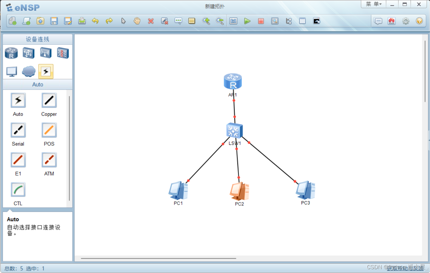
Huawei ENSP simulator configures DHCP for router

奋斗正当时,城链科技战略峰会广州站圆满召开

Methods of improving machine vision system
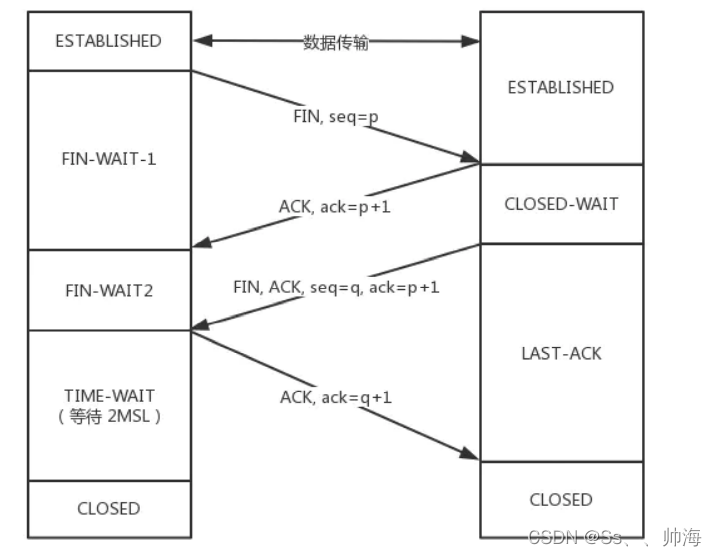
TCP三次握手,四次挥手,你真的了解吗?
随机推荐
Application practice | Shuhai supply chain construction of data center based on Apache Doris
Analysis of maker education technology in the Internet Era
Shutter WebView example
杰理之AD 系列 MIDI 功能说明【篇】
Go language loop statement (3 in Lesson 10)
Kubeadm初始化报错:[ERROR CRI]: container runtime is not running
Flutter 返回按钮的监听
Cadeus has never stopped innovating. Decentralized edge rendering technology makes the metauniverse no longer far away
CAD中能显示打印不显示
MP3是如何诞生的?
redis布隆过滤器
redis03——Redis的网络配置与心跳机制
Redis cache
为什么说不变模式可以提高性能
Flutter TextField示例
Jerry added the process of turning off the touch module before turning it off [chapter]
华为ensp模拟器 给路由器配置DHCP
Jerry's ad series MIDI function description [chapter]
[buuctf.reverse] 151_[FlareOn6]DnsChess
【LeetCode】17、电话号码的字母组合