Deep learning: derivation of shallow neural networks and deep neural networks

I have written several blogs about neural networks before learning machine learning , Recently, I watched the video of Wu Enda's in-depth learning , The neural network is different from before , So take a note .

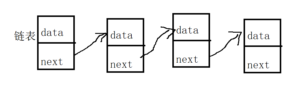
Basic structure and symbol convention

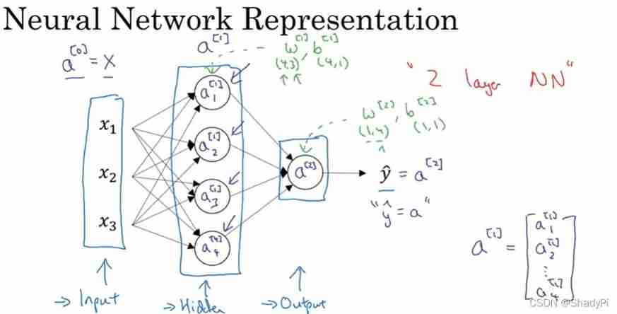
The basic structure is the input layer 、 Hidden layer , Middle layer , Incentive letter $a$ Express , The layer label of the unit is placed in square brackets , The sample number in parentheses , So there is an input layer $x$（$a^{[0]}$）、 Hidden layer $a^{[1]}$ And output layer $a^{[2]}$. Weight is needed in the operation $w$ And offset $b$, The functions in the unit are still logical functions $\sigma (z)=\frac{1}{1+e^{-z}}$.

Declare data matrix $X(n\times m)$, Weight matrices $W^{[l]}(s_l\times s_{l-1})$ And bias matrix $b^{[l]}(s_l\times 1)$, Excitation matrix $A^{[l]}(s_l\times m)$,$n^{[l]}$ It means the first one $l$ The number of cells in the layer , Make
$$A^{[0]}=X=\left[\begin{array}{cccc}|& |& & |\\ x^{(1)}& x^{(2)}& \cdots & x^{(m)}\\ |& |& & |\end{array}\right],W^{[l]}=\left[\begin{array}{ccc}-& w_1^{[l]T}& -\\ -& w_2^{[l]T}& -\\ & \cdots & \\ -& w_{n^{[l]}}^{[l]T}& -\end{array}\right],b^{[l]}=\left[\begin{array}{c}{b}_1^{[l]}\\ b_2^{[l]}\\ ⋮\\ b_{n^{[l]}}^{[l]}\end{array}\right]$$

There are also some supplements that can be seen Neural networks in machine learning .

Spread forward

Yes Neural network vectorization derivation in machine learning Bottoming , Plus forward propagation is relatively simple , Let's go directly to multiple groups of data + Multiple hidden layers .

The middle vector $z^{[l]}$ by
$$z^{[l]}=\left[\begin{array}{c}{z}_1^{[l]}\\ z_2^{[l]}\\ ⋮\\ z_{n^{[l]}}^{[l]}\end{array}\right]=\left[\begin{array}{c}{w}_1^{[l]T}{a}^{[l-1]}+b_1^{[l]}\\ w_2^{[l]T}{a}^{[l-1]}+b_2^{[l]}\\ ⋮\\ w_{n^{[l]}}^{[l]T}{a}^{[l-1]}+b_{n^{[l]}}^{[l]}\end{array}\right]=W^{[l]}{a}^{[l-1]}+b^{[l]}$$
So by the $z^{[l](i)}$ A matrix of $Z^{[l]}$ by
$$Z^{[l]}=\left[\begin{array}{cccc}|& |& & |\\ z^{[l](1)}& z^{[l](2)}& \cdots & z^{[l](m)}\\ |& |& & |\end{array}\right]=W^{[l]}{A}^{[l-1]}+b^{[l]}$$
And the excitation matrix of the hidden layer $A^{[l]}$ Namely
$$A^{[l]}=\left[\begin{array}{cccc}|& |& & |\\ a^{[l](1)}& a^{[l](2)}& \cdots & a^{[l](m)}\\ |& |& & |\end{array}\right]=\sigma (Z^{[l]})=\sigma (W^{[l]}{A}^{[l-1]}+b^{[l]})$$

Other activation functions

Before, our neural networks were all logical functions used by logistic regression , But in fact, there are many better choices in Neural Networks .

tanh function

$$\tanh (z)=\frac{e^z-e^{-z}}{e^z+e^{-z}}$$
The image below ：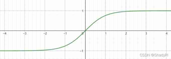

$\tanh$ Functions are almost strictly superior to logical functions , because $\tanh$ Function so that the average value of the excitation is 0 about , This can make the calculation of the next level easier . Except at the output layer , What we expect is $0\sim 1$ Between the output , At this time, we can use logical functions in the output layer .

The derivative of this function is
$${\tanh }^{\prime }(z)=1-(\tanh (z){)}^2$$

ReLU function

But logical functions and $\tanh$ Every function has a problem , That is when the absolute value of coordinates is very large , The gradient of the function becomes very small , In this way, when we run an algorithm similar to gradient descent, the convergence speed will become very slow . and ReLU Function can solve this problem , The expression is
$$\text{ReLU}(z)=\max (0,z)$$
The image is ：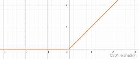

such , as long as $z>0$, The derivative is 1, and $z<0$ The time derivative is 0. Although mathematically $z=0$ There is no derivative at , however $z$ The value is just 0 The probability is very small , And we can artificially define it as 1 or 0, This is harmless in practical application .

In general , If you want to do a binary classification problem , We might use it $\tanh$ function , Add a logic function to the output layer , At other times, it is generally the default ReLU function .

Leaky ReLU

In practice ,ReLU Functions usually perform well , But because the derivative of its negative part is 0, So for this part, its gradient descent rate will be very slow , Although in a network , We will have many positive parts , Make the whole parameters still learn at a faster speed . If you are not at ease , You can also set a smaller slope for the negative part , such as $0.01$, In this way, the activation function is expressed as
$$\text{Leaky ReLU}(z)=\max (0.01z,z)$$

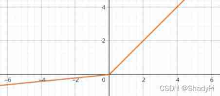
Back propagation

Shallow neural networks

Backward propagation is more complex , Let's first push a shallow neural network ：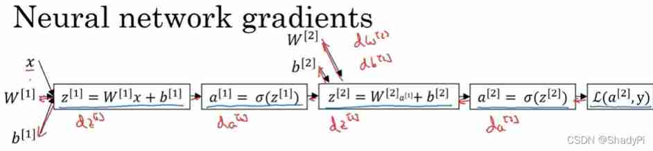

First , For the last cost function , Its value is
$$\mathcal{L}(a^{[2]},y)=-y\log a^{[2]}-(1-y)\log (1-a^{[2]})$$
Yes $a^{[2]}$ Find differentiation , Available
$$\frac{d\mathcal{L}}{d{a}^{[2]}}=-\frac{y}{a^{[2]}}+\frac{1-y}{1-a^{[2]}}$$
be $z^{[2]}$ The differential of the cost function is
$$\frac{d\mathcal{L}}{d{z}^{[2]}}=\frac{d\mathcal{L}}{d{a}^{[2]}}\frac{d{a}^{[2]}}{d{z}^{[2]}}=(-\frac{y}{a^{[2]}}+\frac{1-y}{1-a^{[2]}})a^{[2]}(1-a^{[2]})=a^{[2]}-y$$
Calculated after $\frac{d\mathcal{L}}{d{W}^{[2]}}$ and $\frac{d\mathcal{L}}{d{b}^{[2]}}$ by
$$\begin{gathered} \frac{d\mathcal{L}}{d{W}^{[2]}}=\frac{d\mathcal{L}}{d{z}^{[2]}}{a}^{[1]T} \\ \frac{d\mathcal{L}}{d{b}^{[2]}}=\frac{d\mathcal{L}}{d{z}^{[2]}} \end{gathered}$$
Now the derivation is half done , Let's calculate again $a^{[1]}$ The derivative of is
$$\frac{d\mathcal{L}}{d{a}^{[1]}}=W^{[2]T}\frac{d\mathcal{L}}{d{z}^{[2]}}$$
because $z^{[2]}$ yes $n^{[2]}\times 1$ Of ,$W^{[2]}$ yes $n^{[2]}\times n^{[1]}$ Of , So it needs to be transposed here . after , Ask again for $z^{[1]}$ The derivative of , Just multiply this by $\frac{d{a}^{[1]}}{d{z}^{[1]}}$（$\ast$ Indicates bitwise multiplication ）：
$$\frac{d\mathcal{L}}{d{z}^{[1]}}=W^{[2]T}\frac{d\mathcal{L}}{d{z}^{[2]}}\ast g^{[1{]}^{\prime }}(z^{[1]})$$
And calculation $\frac{d\mathcal{L}}{d{W}^{[1]}}$ and $\frac{d\mathcal{L}}{d{b}^{[1]}}$ Process and Chapter 2 The layers are almost identical ：
$$\begin{gathered} \frac{d\mathcal{L}}{d{W}^{[1]}}=\frac{d\mathcal{L}}{d{z}^{[1]}}{a}^{[0]T} \\ \frac{d\mathcal{L}}{d{b}^{[1]}}=\frac{d\mathcal{L}}{d{z}^{[1]}} \end{gathered}$$
The above derivation is for a single sample , Backward propagation is required for multiple samples , Stack the sample column vectors by column , You can apply the results derived above , It's all $n^{[l]}\times 1$ The matrix becomes $n^{[l]}\times m$, then $b$ The vector needs to be summed once in the horizontal direction （ To simplify the expression , We use it $d{Z}^{[2]}$ According to matrix $Z^{[2]}$ The result of deriving the cost function , Other matrices are the same ）：
$$\begin{array}{rl}& d{Z}^{[2]}=(A^{[2]}-Y)\\ & d{W}^{[2]}=\frac{1}{m}d{Z}^{[2]}{A}^{[1]T}\\ & d{b}^{[2]}=\frac{1}{m}np.sum(d{Z}^{[2]},axis=1,keepdims=True)\\ & d{Z}^{[1]}=W^{[2]T}d{Z}^{[2]}\ast g^{[1{]}^{\prime }}(Z^{[1]})\\ & d{W}^{[1]}=\frac{1}{m}d{Z}^{[1]}{X}^T\\ & d{b}^{[1]}=\frac{1}{m}np.sum(d{Z}^{[1]},axis=1,keepdims=True)\end{array}$$keepdims The function of is to let Python Don't put our column vector (n,1) Become rank 1 Matrix (n,), That could lead to hard to find bug.

Deep neural network

The shallow network above has only two layers , And for complex problems , Increase the number of layers of the network （ depth ） It is much more effective than forcing nodes to be added in a hidden layer , So we need to transform the above derivation into a more general form , That is, the following four formulas ：
$$\begin{array}{rl}& d{Z}^{[l]}=d{A}^{[l]}\ast g^{[l{]}^{\prime }}(Z^{[l]})\\ & d{W}^{[l]}=\frac{1}{m}d{Z}^{[l]}{A}^{[l-1]T}\\ & d{b}^{[l]}=\frac{1}{m}np.sum(d{Z}^{[l]},axis=1,keepdims=True)\\ & d{A}^{[l-1]}=W^{[l]T}d{Z}^{[l]}\end{array}$$
Initial input $d{A}^{[L]}$ Determined by the excitation function of the output node , about $m$ Group samples , Its value is
$$d{A}^{[L]}=\left[\begin{array}{cccc}\frac{d\mathcal{L}}{d{a}^{[L](1)}}& \frac{d\mathcal{L}}{d{a}^{[L](2)}}& \cdots & \frac{d\mathcal{L}}{d{a}^{[L](m)}}\end{array}\right]$$

From the above formula , We can input $d{A}^{[l]}$, Output $d{A}^{[l-1]}$, At the same time, calculate the weight of each layer and the gradient of offset .