当前位置:网站首页>Linear programming matlab
Linear programming matlab
2022-07-06 02:50:00 【Foreign rookie】
Catalog
Two 、 Mathematical form expression of concept
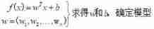
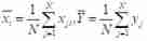
3、 ... and 、 determine w and b
2. normalization 、 Standardization
1. Solve the equation directly
2. Least square method (least square method) solve :
4. Evaluating regression models
Four 、regress Linear regression command
1. Adjust the function to solve the equation
2. Plot the original and predicted values
5、 ... and 、matlab color table
2、 Functions that generate standard palettes
One 、 Basic concepts
linear (linear):
It refers to the proportion between quantity and quantity 、 In a straight line , Represent regular and smooth motion in space and time , The first derivative is constant
nonlinear (non-linear):
It means not in proportion 、 A non-linear relationship , Represents irregular movement and mutation , The first derivative is not constant .
A linear example :
data : Salary and age (2 Features )
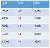
The goal is : Predict how much the bank will lend me ( label )
consider : Both salary and age will affect the final result of bank loans , How much influence do they have respectively ?( Parameters )
Popular explanation :
x1,x2 It's our two characteristics ( Age 、 Wages ),y It's how much money the bank will eventually lend us
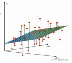
Find the most suitable line ( Imagine a high dimension ) To best fit our data points
Here comes the mathematical form
Two 、 Mathematical form expression of concept
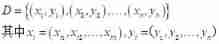
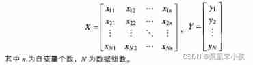
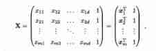
Given data set :
Matrix form of data :
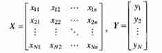
Linear model (linear model) Try to learn a function to predict through the linear combination of attribute combination , namely
![]()
use Vector form It's written in :
Linear regression (linear regression) Try to learn a linear model to predict the real value output mark as accurately as possible
![]()
3、 ... and 、 determine w and b
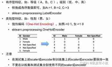
For discrete attributes :
If between attributes There is “ order ” Relationship , It can be converted into continuous values by continuity .
If between attributes non-existent “ order ” Relationship , It's translated into k Dimension vector .
1. Read or input data
matlab No need to import libraries , Direct reference function csvread Read csv Data files
Let's first look at csv Data import
%  Reference function  csvread  Read csv Data files

data = csvread(' route ',1,0) # From the second line , The first 0 Column read data
After reading the data, the sum is X, What is the Y
# matlab from 1 Start counting , As it is
X = data[:,1:4] # 1 To 4 List all the data, that is, the actual 1 To 4 Column
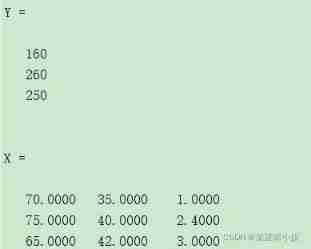
Y = data[:, 6] # The first 6 List all the data, that is, the actual number 6 Column Next Let's see what we build matrix How to read data
Y=[160
   260
   250];

X=[70,35,1
 75,40,2.4
 65,42,3];
return :
Speaking of matrices , By the way
Knowledge about creating matrices :
(1) ones() function : All are 1 Matrix ,ones(n): produce n*n The whole of dimension 1 matrix ,ones(m,n): produce m*n The whole of dimension 1 matrix ;
(2) zeros() function : All are 0 Matrix ;
(3) rand() function : Produced in (0,1) Interval uniformly distributed random matrix ;
(4) eye() function : Generate unit matrix ;
(5) randn() function : The average production is 0, The variance of 1 Standard normal distribution random matrix .
2. normalization 、 Standardization
2.1 mean value
# MATLAB Direct reference mean() Function is good
X_mean = mean(X)
Y_mean = mean(Y)
1. mean: Calculate the vector mean .mean(x,1) Column vector mean ,mean(x,2) Row vector mean . mean2(x) Matrix mean .
2. std: Calculate the mean square deviation of the vector ,std(x,0,1) Column vector mean square deviation ,std(x,0,2) Mean square deviation of row vector . std2(x) Matrix mean square deviation
3. var: Calculate vector variance ,var(x)
4. sse: The sum of the squares of the errors ,sse(x). The more close to 0, It shows that the better the fitting , The more successful the data prediction .
5. mse: Sum of squares of mean square deviation ,mse(x)=sse(x)/N. It means the same thing sse
6. R-square: Determine the coefficient . The coefficient of determination represents the quality of a fitting through the change of data . From the above expression, we can know “ Determine the coefficient ” The normal value range of is [0 1], The closer the 1, Show that the variables of the equation are y The better the ability to explain , This model fits the data well .
To be sure w and b, First, we should decide whether to normalize or standardize the data according to the situation
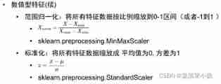
2.2 normalization
% normalization

X=[70,35,1
 75,40,2.4
 65,42,3];
for X=X
    MappedX = (X-min(X))/(max(X)-min(X))
end
% Use functions mapminmax
% default map The scope is [-1, 1], So if you need to [0, 1], Then provide parameters in such a format :
MappedData = mapminmax(OriginalData, 0, 1);% Normalize by line only , If it's a matrix , Then each row is normalized , If you need to normalize the entire matrix
FlattenedData = OriginalData(:)'; % Expand the matrix into a column , Then transpose to one line .
MappedFlattened = mapminmax(FlattenedData, 0, 1); % normalization .
% Restore to the original matrix form . There is no need to transpose back here , because reshape It happens to be reordering by column
MappedData = reshape(MappedFlattened, size(OriginalData)); 2.3 Standardization
% z-score  Standardization
%  The new data =( The original data - mean value )/ Standard deviation
%  After standardization ,X The value range of the element in is a real number .

X=zscore(X)
3. solve w and b
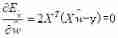
1. Solve the equation directly
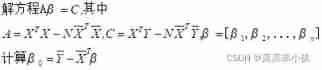
N = length(Y);

A = X'*X-(N*X_mean'*X_mean);
C=X'*Y - (N*X_mean'*Y_mean);
B = (A^-1*C).'
2. Least square method (least square method) solve :
Put the data set D To express as a m*(d+1) Matrix of size X, Each line corresponds to an example , Change career d The elements correspond to the... Of the example d Attribute values , It is better to set an element to 1, namely
A=[1 2 3;4 5 6;7 8 9];
B = ones(3,1) % Generate 3 That's ok 1 Column 1 matrix
% B=[1;1;1];  % Three lines in all , use “;” Separate
A_column=[A B];
display(A_column);% Output results
When X^TX Is a full rank matrix (full-rank matrix) Or walking matrix (positive definite matrix) when , Make
obtain
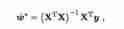
w = (X'*X)^-1*X'*Y % The coefficient of the variable
w0 = Y_mean - X_mean*w % constant
among (X^TX)^-l It's a matrix (X^TX) The inverse matrix . Make xi = (xi ,l) , Then the final multiple linear regression model is
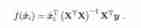
YY = X*w+w0 %Y The estimate of 4. Evaluating regression models
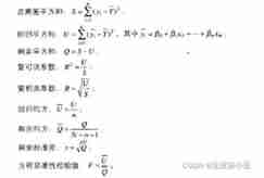
% Sum of squares of deviations
S = var(Y);
fprintf(' Sum of squares of deviations S=:%d\n',S)
% Sum of regression squares
U = var(YY);
fprintf(' Sum of regression squares U=:%d\n',U)
% The sum of the remaining squares
Q=S-U;
fprintf(' The sum of the remaining squares Q=:%d\n',Q)
% Complex determinate coefficient
R2 = U/S;
fprintf(' Complex determinate coefficient R2=:%d\n',R2)
% Negative correlation coefficient
R = sqrt(U/S);
fprintf(' Complex correlation coefficient R=:%d\n',R)
% Regression mean square
% n= X_mean  The number of
UU = U/n;
fprintf(' Regression mean square =:%d\n',UU)
% Residual mean square
% N= Y The number of
QQ = Q/(N-n-1);
fprintf(' Residual mean square =:%d\n',QQ)
% Residual standard deviation
s = sqrt(QQ);
fprintf(' Residual standard deviation s=:%d\n',s)
% Equation significance test value
F = UU/QQ;
fprintf(' Variance significance test value F=:%d\n',F)
Four 、regress Linear regression command
For univariate and multivariate linear regression , It's essentially the least squares method . stay Matlab 2014a in , Input help regress , Will pop up and regress Information about
Invocation format :
- B = regress(Y,X)
- [B,BINT] = regress(Y,X)
- [B,BINT,R] = regress(Y,X)
- [B,BINT,R,RINT] = regress(Y,X)
- B,BINT,R,RINT,STATS] = regress(Y,X)
- [...] = regress(Y,X,ALPHA)
Parameter interpretation :
- B: Regression coefficient , It's a vector (“the vector B of regression coefficients in the linear model Y = X*B”).
- BINT: Interval estimates of regression coefficients (“a matrix BINT of 95% confidence intervals for B”).
- R: residual ( “a vector R of residuals”).
- RINT: confidence interval (“a matrix RINT of intervals that can be used to diagnose outliers”).
- STATS: Statistics used to test the regression model . Yes 4 A numerical : Determination factor R^2,F Statistics Observations , Tested p Value , Estimation of error variance .
- ALPHA: Significance level ( Default value if missing 0.05).
1. Adjust the function to solve the equation
%  Equation solving function uses
[b,bint,r,rint,stats] = regress(Y,X);
2. Plot the original and predicted values
x = 1:1:N;
plot(x,Y,'-*b',x,YY,'-or'); % linear , Color , Mark

% hold on; % It means to continue painting on the same picture
% title('x'); % Named title
% axis([0 1 0 10]) %  Set the coordinate axis in the specified interval
% xlabel('t'); % name x Axis
% ylabel('x'); % name y Axis
% grid on % Show axis gridlines
% legend('Y','YY'); %* Annotate ,2 What do the lines represent *
3. Draw residual diagram :
figure % create a window
rcoolot(r,rint) % Draw a residual diagram
5、 ... and 、matlab color table
Linetype | explain | Marker | explain | Color | explain |
- | Solid line ( Default ) | + | The plus sign | r | Red |
-- | Double line | o | The hollow circle | g | green |
: | Dotted line | * | asterisk | b | Blue |
:. | Point line | . | Solid round | c | Turquoise |
x | The cross sign | m | Magenta | ||
s(square) | Square | y | yellow | ||
d | The diamond | k | black | ||
^ | Top triangle | w | white | ||
v | Lower triangle | ||||
> | Right triangle | ||||
< | Left triangle | ||||
p(pentagram) | Five-pointed star | ||||
h(hexagram) | hexagon | ||||
| square | Square | ||||
| pentagram | Pentagonal | ||||
| hexagram | hexagon |
6、 ... and 、matlab palette
1、 Common colors RGB value
--------------------------------------------
Color R G B Color R G B
--------------------------------------------
black 0 0 1 Magenta 1 0 1
white 1 1 1 Bluish green 0 1 1
red 1 0 0 Sky blue 0.67 0 1
green 0 1 0 Orange 1 0.50
blue 0 0 1 Crimson 0.5 0 0
yellow 1 1 0 ash 0.5 0.50.5
--------------------------------------------
️ Be careful :MATLAB Color intensity of palette [0,1],0 Represents the darkest ,1 Represents the brightest .
2、 Functions that generate standard palettes
-------------------------------------------------
Function name palette
-------------------------------------------------
Hsv Color saturation , Start in red , And end in red
Hot black - Red - yellow - white
Cool Cyan and magenta
Pink The color of pink
Gray Linear grayscale
Bone Grayscale with blue
Jet Hsv A deformation of , Start with blue , End in blue
Copper Linear copper color
Prim prism , Alternating red 、 Orange 、 yellow 、 Green and sky blue
Flag Alternating red 、 white 、 Blue and black
--------------------------------------------------
By default , Call the above function to generate a 64×3 My palette , The user can also specify the palette size .
边栏推荐
- 微软语音合成助手 v1.3 文本转语音工具,真实语音AI生成器
- Déduisez la question d'aujourd'hui - 729. Mon emploi du temps I
- 深度解析链动2+1模式,颠覆传统卖货思维?
- Dachang image library
- 【若依(ruoyi)】启用迷你导航栏
- C语言sizeof和strlen的区别
- Follow the mouse's angle and keyboard events
- 会员积分营销系统操作的时候怎样提升消费者的积极性?
- Six stone management: why should leaders ignore product quality
- Gifcam v7.0 minimalist GIF animation recording tool Chinese single file version
猜你喜欢
![[ruoyi] set theme style](/img/e9/6a6b7113faed16c3b439230806320b.png)
[ruoyi] set theme style
![[Yunju entrepreneurial foundation notes] Chapter II entrepreneur test 22](/img/e0/21367eeaeca10c0a2f2aab3a4fa1fb.jpg)
[Yunju entrepreneurial foundation notes] Chapter II entrepreneur test 22
![[Chongqing Guangdong education] higher mathematics I reference materials of Southwest Petroleum University](/img/0f/520242492524522c887b6576463566.jpg)
[Chongqing Guangdong education] higher mathematics I reference materials of Southwest Petroleum University
![[Yunju entrepreneurial foundation notes] Chapter II entrepreneur test 17](/img/85/2635afeb2edeb0f308045edd1f3431.jpg)
[Yunju entrepreneurial foundation notes] Chapter II entrepreneur test 17
Fault analysis | analysis of an example of MySQL running out of host memory

2022.02.13
A copy can also produce flowers
![[Yunju entrepreneurial foundation notes] Chapter II entrepreneur test 10](/img/89/1c2f98973b79e8d181c10d7796fbb5.jpg)
[Yunju entrepreneurial foundation notes] Chapter II entrepreneur test 10
MySQL winter vacation self-study 2022 11 (9)
C # create self host webservice
随机推荐
[ruoyi] enable Mini navigation bar
Redis skip table
How to read excel, PDF and JSON files in R language?
Yyds dry inventory comparison of several database storage engines
华为、H3C、思科命令对比,思维导图形式从基础、交换、路由三大方向介绍【转自微信公众号网络技术联盟站】
Li Kou today's question -729 My schedule I
"Hands on learning in depth" Chapter 2 - preparatory knowledge_ 2.3 linear algebra_ Learning thinking and exercise answers
【若依(ruoyi)】启用迷你导航栏
XSS challenges绕过防护策略进行 XSS 注入
Maturity of master data management (MDM)
Installation and use tutorial of cobaltstrike-4.4-k8 modified version
[Digital IC manual tearing code] Verilog asynchronous reset synchronous release | topic | principle | design | simulation
Apt installation ZABBIX
Referenceerror: primordials is not defined error resolution
1. Dynamic parameters of function: *args, **kwargs
解决:AttributeError: ‘str‘ object has no attribute ‘decode‘
Microservice registration and discovery
【Kubernetes 系列】一文學會Kubernetes Service安全的暴露應用
Taobao focus map layout practice
[Chongqing Guangdong education] higher mathematics I reference materials of Southwest Petroleum University