当前位置:网站首页>Label propagation
Label propagation
2022-07-02 07:39:00 【Xiao Chen who wants money】
Recently, I am studying the semi supervised algorithm of time series , See this algorithm , It was recorded .
Reprinted from : Tag propagation algorithm (Label Propagation) And Python Realization _zouxy09 The column -CSDN Blog _ Tag propagation algorithm
Semi-supervised learning (Semi-supervised learning) The occasion to play a role is : Some of your data have label, Some don't . And most of them don't , Only a few have label. Semi supervised learning algorithm will make full use of unlabeled Data to capture the potential distribution of our entire data . It is based on three assumptions :
1)Smoothness Smoothing hypothesis : Similar data have the same label.
2)Cluster Clustering hypothesis : Data under the same cluster have the same label.
3)Manifold Manifold hypothesis : Data in the same manifold structure have the same label.
Tag propagation algorithm (label propagation) The core idea of is very simple : Similar data should have the same label.LP The algorithm consists of two steps :1) Construct similarity matrix (affinity matrix);2) Spread it bravely .
label propagation Is a graph based algorithm . Graph is based on vertices and edges , Each vertex is a sample , All vertices include labeled samples and unlabeled samples ; Edges represent vertices i To the top j Probability , In other words, the vertex i To the top j The similarity .

here ,α It's a superscript .
Another very common method of graph construction is knn chart , That is, only for each node k Nearest neighbor weight , The other is 0, That is, there is no edge , So it's a sparse similarity matrix .
The label propagation algorithm is very simple : Propagate through the edges between nodes label. The more weight an edge has , Indicates that the more similar two nodes are , that label The easier it is to spread the past . Let's define a NxN Probability transition matrix P:
Pij Represents slave node i Transfer to node j Probability . Suppose there is C Class and L individual labeled sample , Let's define a LxC Of label matrix YL, The first i Line representation i Labels of samples indicate vectors , That is, if the second i The categories of samples are j, Then the No j Elements are 1, For the other 0. Again , We also give U individual unlabeled One sample UxC Of label matrix YU. Merge them , We get a NxC Of soft label matrix F=[YL;YU].soft label It means , We keep the sample i The probability of belonging to each category , Not mutually exclusive , This sample is based on probability 1 Only belong to one class . Yes, of course , Finally determine this sample i Of the category , Is to take max That is, the class with the greatest probability is its class . that F There's a YU, It didn't know at first , What is the initial value ? It doesn't matter , Just set any value .
Come out , ordinary LP Algorithm is as follows :
1) Execute propagation :F=PF
2) Reset F in labeled The label of the sample :FL=YL
3) Repeat step 1) and 2) until F convergence .
step 1) That's to put the matrix P And matrices F Multiply , This step , Each node will have its own label With P The determined probability is propagated to other nodes . If the two nodes are more similar ( The closer the distance in European space ), So the other side's label The easier it is to be label give , It's easier to form gangs . step 2) It's critical , because labeled Data label It's predetermined , It cannot be taken away , So after each transmission , It has to return to its original label. With labeled The data will continue to own label Spread it out , The last class boundary will cross the high-density region , And stay in low-density intervals . Equivalent to each different category labeled The sample divides the sphere of influence .
2.3、 Transformed LP Algorithm
We know , We calculate one for each iteration soft label matrix F=[YL;YU], however YL It is known. , It's useless to calculate it , Steps in 2) When , We have to get it back . All we care about is YU, Can we just calculate YU Well ?Yes. We will matrix P Make the following division :

Now , Our algorithm is just an operation :

Iterate the above steps until convergence ok 了 , Isn't it very cool. You can see FU Not only depends on labeled Label of data and its transfer probability , It depends unlabeled Current data label And transition probability . therefore LP The algorithm can be used additionally unlabeled Distribution characteristics of data .
The convergence of this algorithm is also very easy to prove , See references for details [1]. actually , It can converge to a convex solution :

So we can also solve it directly in this way , To get the final YU. But in the actual application process , Because matrix inversion requires O(n3) Complexity , So if unlabeled There's a lot of data , that I – PUU The inversion of the matrix will be very time-consuming , Therefore, at this time, we usually choose iterative algorithm to realize .
#***************************************************************************
#*
#* Description: label propagation
#* Author: Zou Xiaoyi ([email protected])
#* Date:   2015-10-15
#* HomePage: http://blog.csdn.net/zouxy09
#*
#**************************************************************************

import time
import numpy as np

# return k neighbors index
def navie_knn(dataSet, query, k):
    numSamples = dataSet.shape[0]

    ## step 1: calculate Euclidean distance
    diff = np.tile(query, (numSamples, 1)) - dataSet
    squaredDiff = diff ** 2
    squaredDist = np.sum(squaredDiff, axis = 1) # sum is performed by row

    ## step 2: sort the distance
    sortedDistIndices = np.argsort(squaredDist)
    if k > len(sortedDistIndices):
        k = len(sortedDistIndices)

    return sortedDistIndices[0:k]


# build a big graph (normalized weight matrix)
def buildGraph(MatX, kernel_type, rbf_sigma = None, knn_num_neighbors = None):
    num_samples = MatX.shape[0]
    affinity_matrix = np.zeros((num_samples, num_samples), np.float32)
    if kernel_type == 'rbf':
        if rbf_sigma == None:
            raise ValueError('You should input a sigma of rbf kernel!')
        for i in xrange(num_samples):
            row_sum = 0.0
            for j in xrange(num_samples):
                diff = MatX[i, :] - MatX[j, :]
                affinity_matrix[i][j] = np.exp(sum(diff**2) / (-2.0 * rbf_sigma**2))
                row_sum += affinity_matrix[i][j]
            affinity_matrix[i][:] /= row_sum
    elif kernel_type == 'knn':
        if knn_num_neighbors == None:
            raise ValueError('You should input a k of knn kernel!')
        for i in xrange(num_samples):
            k_neighbors = navie_knn(MatX, MatX[i, :], knn_num_neighbors)
            affinity_matrix[i][k_neighbors] = 1.0 / knn_num_neighbors
    else:
        raise NameError('Not support kernel type! You can use knn or rbf!')

    return affinity_matrix


# label propagation
def labelPropagation(Mat_Label, Mat_Unlabel, labels, kernel_type = 'rbf', rbf_sigma = 1.5, \
                    knn_num_neighbors = 10, max_iter = 500, tol = 1e-3):
    # initialize
    num_label_samples = Mat_Label.shape[0]
    num_unlabel_samples = Mat_Unlabel.shape[0]
    num_samples = num_label_samples + num_unlabel_samples
    labels_list = np.unique(labels)
    num_classes = len(labels_list)

    MatX = np.vstack((Mat_Label, Mat_Unlabel))
    clamp_data_label = np.zeros((num_label_samples, num_classes), np.float32)
    for i in xrange(num_label_samples):
        clamp_data_label[i][labels[i]] = 1.0

    label_function = np.zeros((num_samples, num_classes), np.float32)
    label_function[0 : num_label_samples] = clamp_data_label
    label_function[num_label_samples : num_samples] = -1

    # graph construction
    affinity_matrix = buildGraph(MatX, kernel_type, rbf_sigma, knn_num_neighbors)

    # start to propagation
    iter = 0; pre_label_function = np.zeros((num_samples, num_classes), np.float32)
    changed = np.abs(pre_label_function - label_function).sum()
    while iter < max_iter and changed > tol:
        if iter % 1 == 0:
            print "---> Iteration %d/%d, changed: %f" % (iter, max_iter, changed)
        pre_label_function = label_function
        iter += 1

        # propagation
        label_function = np.dot(affinity_matrix, label_function)

        # clamp
        label_function[0 : num_label_samples] = clamp_data_label

        # check converge
        changed = np.abs(pre_label_function - label_function).sum()

    # get terminate label of unlabeled data
    unlabel_data_labels = np.zeros(num_unlabel_samples)
    for i in xrange(num_unlabel_samples):
        unlabel_data_labels[i] = np.argmax(label_function[i+num_label_samples])

return unlabel_data_labels边栏推荐
- Cognitive science popularization of middle-aged people
- 优化方法:常用数学符号的含义
- 【Paper Reading】
- Using compose to realize visible scrollbar
- Feeling after reading "agile and tidy way: return to origin"
- 【信息检索导论】第一章 布尔检索
- 【Mixup】《Mixup:Beyond Empirical Risk Minimization》
- [tricks] whiteningbert: an easy unsupervised sentence embedding approach
- 【论文介绍】R-Drop: Regularized Dropout for Neural Networks
- mmdetection训练自己的数据集--CVAT标注文件导出coco格式及相关操作
猜你喜欢

Ding Dong, here comes the redis om object mapping framework

Faster-ILOD、maskrcnn_benchmark安装过程及遇到问题
基于onnxruntime的YOLOv5单张图片检测实现

The difference and understanding between generative model and discriminant model
![[CVPR‘22 Oral2] TAN: Temporal Alignment Networks for Long-term Video](/img/bc/c54f1f12867dc22592cadd5a43df60.png)
[CVPR‘22 Oral2] TAN: Temporal Alignment Networks for Long-term Video
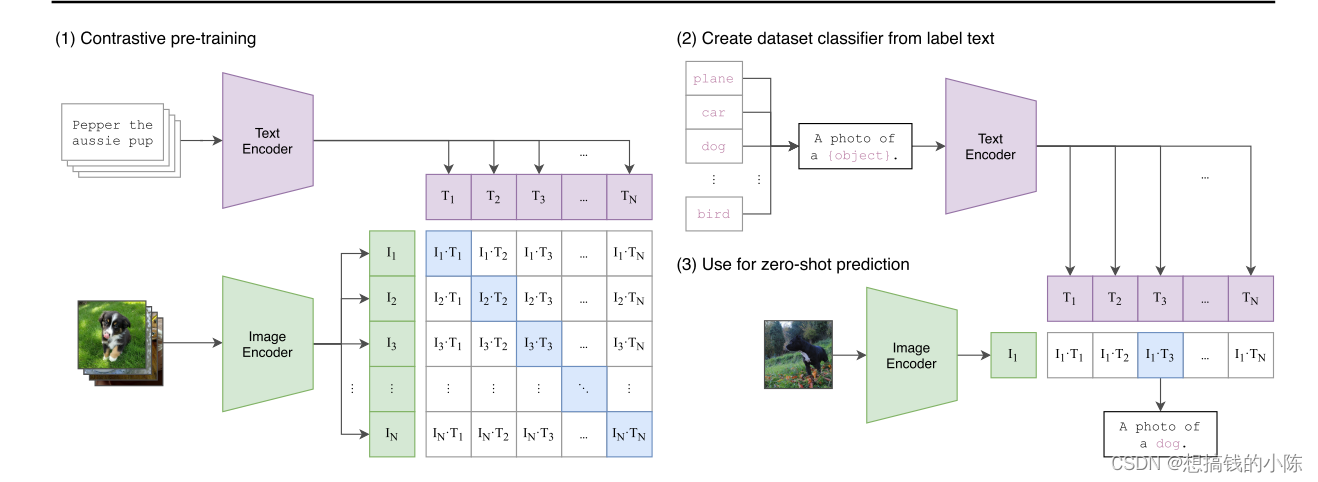
【多模态】CLIP模型
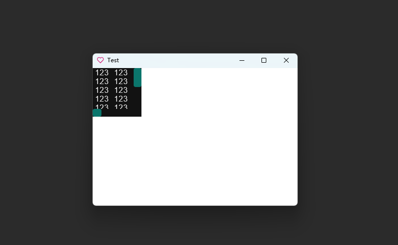
使用 Compose 实现可见 ScrollBar
![[tricks] whiteningbert: an easy unsupervised sentence embedding approach](/img/8e/3460fed55f2a21f8178e7b6bf77d56.png)
[tricks] whiteningbert: an easy unsupervised sentence embedding approach
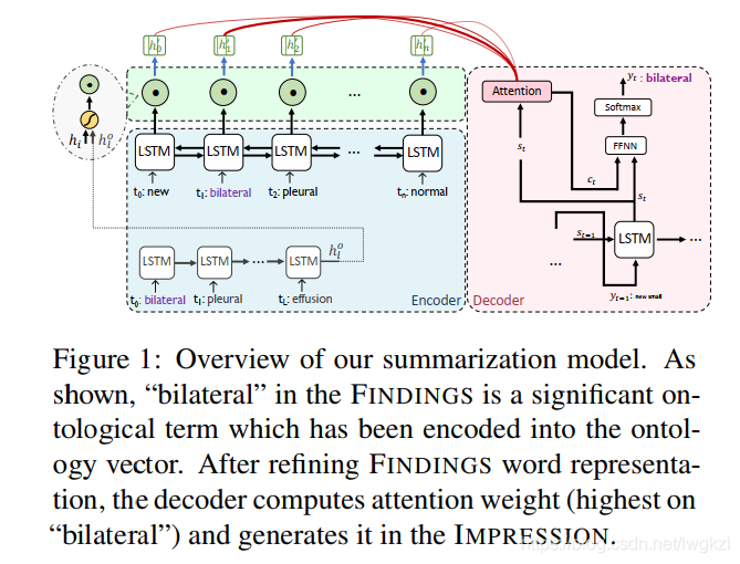
【MEDICAL】Attend to Medical Ontologies: Content Selection for Clinical Abstractive Summarization
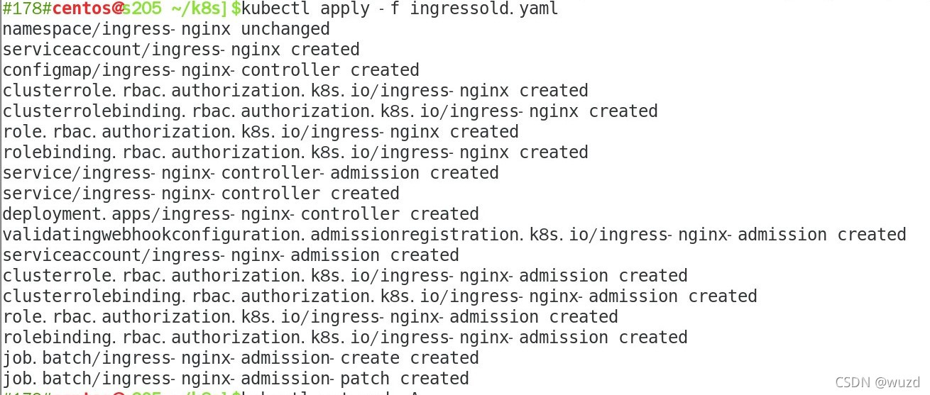
Yaml file of ingress controller 0.47.0
随机推荐
Open failed: enoent (no such file or directory) / (operation not permitted)
Faster-ILOD、maskrcnn_benchmark安装过程及遇到问题
常见的机器学习相关评价指标
PointNet原理证明与理解
Conda 创建,复制,分享虚拟环境
【BERT,GPT+KG调研】Pretrain model融合knowledge的论文集锦
Spark SQL task performance optimization (basic)
Drawing mechanism of view (I)
Regular expressions in MySQL
Alpha Beta Pruning in Adversarial Search
生成模型与判别模型的区别与理解
MMDetection安装问题
一份Slide两张表格带你快速了解目标检测
MySQL has no collation factor of order by
PHP returns the corresponding key value according to the value in the two-dimensional array
Classloader and parental delegation mechanism
【信息检索导论】第七章搜索系统中的评分计算
【Programming】
ERNIE1.0 与 ERNIE2.0 论文解读
【Torch】最简洁logging使用指南