Based on the least squares linear regression equation coefficient estimation

I. Description of the problem

Unary linear regression analysis is a very simple and very basic regression theory, which can be used to describe the change trend of the linear relationship between two variables, and then predict the data at the unknown point.
Regression analysis is to determine the regression function (equation) according to the change trend of the known data, in which the regression coefficient is to be determined, and then some numerical methods or statistical methods are used to estimate the regression coefficient.
Univariate linear regression analysis is to estimate the coefficients k and b in the equation y=kx+b. The common methods are: computational mathematics - least squares method, statistical method - maximum likelihood estimation method, machine learningMethods - perceptrons, etc., in addition, you can use the operation of the matrix (in fact, it is only the minimum value solution) to solve it directly.
This article takes the data of y = 2x + 1 and y = -2x + 5 for fitting as an example, and gives the method of estimating the regression coefficient by the least square method and its realization in matlab.

II. Mathematical derivation

Problem description:
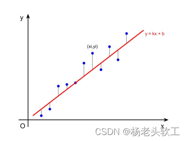
As shown above, assuming the known data points (xi,yi), i=1...n, and the observation of the scatter plot basically satisfies the linear trend, according to which the function expression of the red straight line is obtained.
As shown in the figure above, the least squares method is to estimate the undetermined coefficients in the regression function by using the minimum sum of the squares of the distances from the known point represented by the black line segment to the regression curve.
The formula is derived as follows:
Substitute (xi,yi) into y=kx+b to get: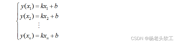

Construct least squares function (sum of squared distances):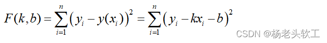

Take the partial derivatives for k and b respectively: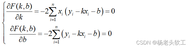

Divide both ends of the above equation by the number of data points n to get: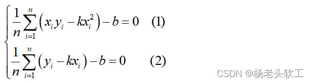

Equation (2) can be further transformed into: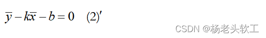

where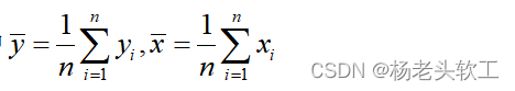

Substitute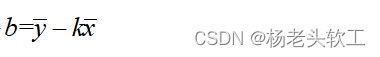

into (1) to get:

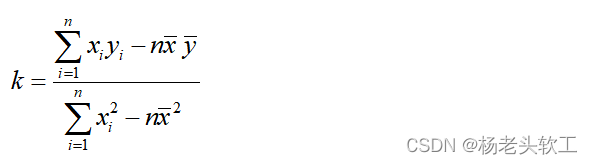
Substitute k into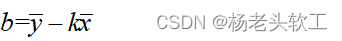

to get coefficient b, so far, the two coefficients in the regression equation are calculated.
3. Matlab program
1. Interpret the changing trend of the curve according to the scatter plot

trainX = linspace( 0, 2, 50 );trainY = 2 * trainX + 1 + randn( size( trainX ) )*0.4;plot( trainX, trainY, 'b.', 'markersize', 20 )

As shown below:

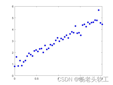
From the distribution of points in the figure, we can see that the basicIt shows a linear growth trend, so consider using y=kx+b to fit this set of data.
2. The regression coefficient is calculated as follows:

n = length( trainX );xu = sum( trainX ) / n;yu = sum( trainY ) / n;k1 = sum( trainX .* trainY ) - n * xu * yu;k2 = sum( trainX .* trainX ) - n * xu * xu;k = k1 / k2;b = yu - k * xu;

The calculation result is:
K = 1.8467, b = 1.2669
3. The complete code is as follows:

% Use the least squares method to estimate the coefficients k and b in the linear regression function y = kx + bclear allclc% Generate training datatrainX = linspace( 0, 2, 50 );trainY = 2 * trainX + 1 + randn( size( trainX ) )*0.4;% draw a scatter plotplot( trainX, trainY, 'b.', 'markersize', 20 )% estimated regression coefficientsn = length( trainX );xu = sum( trainX ) / n;yu = sum( trainY ) / n;k1 = sum( trainX .* trainY ) - n * xu * yu;k2 = sum( trainX .* trainX ) - n * xu * xu;k = k1 / k2;b = yu - k * xu;% draw the regression function curve (straight line)hold onx = [ -0.5 ; 2.5 ];y = k * x + b; % regression equationplot( x, y, 'r', 'LineWidth', 2 );title( 'LSM : y = 2x + 1' )axis( [ -0.5, 2.5, -1, 7 ] )

The fitting results are as follows: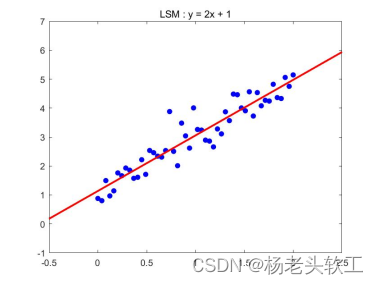

Modify statement"trainY = 2 * trainX + 1 + randn( size( trainX ) )*0.1;”
are different functional relationships, and different regression curves can be obtained.For example, modify it to
"trainY = -2 * trainX -5 + randn( size( trainX ) )*0.4;"
to get the following fitted image: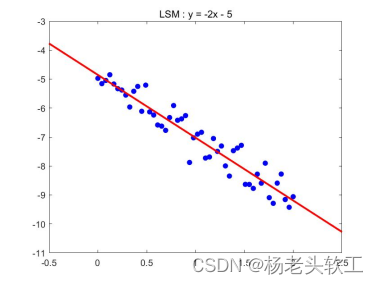

4. Supplementary note
The least squares method is a very good method for estimating regression by finding the extreme value of a function.The method of parameters in the equation, in fact, although the objective function of the regression coefficient estimated by the maximum likelihood method is different, the results are the same as those estimated directly by the least squares method.