当前位置:网站首页>The second official example analysis of the MOOSE platform - about creating a Kernel and solving the convection-diffusion equation
The second official example analysis of the MOOSE platform - about creating a Kernel and solving the convection-diffusion equation
2022-08-04 06:19:00 【nuomi666】
There may be errors,欢迎大家批评指正
一、例子介绍
This article USES the website provides the second example( MOOSE|EX02),This example of solving the equation is in diffusion equation(泊松方程)Above add advection term,Advection velocity v ⃗ \vec{v} v在 z z zDirections for 1 1 1,否则为零.The boundary conditions usingDirichlet边界.On the bottom of the solution domain u = 1 u=1 u=1 ,在顶部 u = 0 u=0 u=0 ,In the rest of the other on the border ∇ u ⋅ n ^ = 0 \nabla u \cdot \hat{n} = 0 ∇u⋅n^=0,其中 n ^ \hat{n} n^Is a normal vector boundary.
− ∇ ⋅ ∇ u + v ⃗ ⋅ ∇ u = 0 ∈ Ω u = 1 ∈ ∂ Ω b o t t o m u = 0 ∈ ∂ Ω t o p ∇ u ⋅ n ^ = 0 ∈ ∂ Ω o t h e r (1.1) \begin{aligned} -\nabla \cdot \nabla u + \vec{v} \cdot \nabla u&=0 && \quad \in \Omega \\ u &= 1 && \quad \in \partial \Omega_{bottom} \\ u &= 0 && \quad \in \partial \Omega_{top}\\ \nabla u \cdot \hat{n}& = 0 && \quad \in \partial \Omega_{other} \end{aligned} \tag{1.1} −∇⋅∇u+v⋅∇uuu∇u⋅n^=0=1=0=0∈Ω∈∂Ωbottom∈∂Ωtop∈∂Ωother(1.1)
二、FEM
1、Generate a weak form
a.On both sides of the equation and take the test function ψ \psi ψ
ψ ( − ∇ ⋅ ∇ u ) + ψ ( v ⃗ ⋅ ∇ u ) = 0 ψ , u ∈ V (2.1) \psi(-\nabla \cdot \nabla u) + \psi (\vec{v} \cdot \nabla u )=0 \quad \quad \psi,u \in V \tag{2.1} ψ(−∇⋅∇u)+ψ(v⋅∇u)=0ψ,u∈V(2.1)
这里 V = H 1 ( Ω ) V =H^{1}{(\Omega)} V=H1(Ω)
b.On the whole solution domain Ω \Omega Ω积分
− ∫ Ω ψ ( ∇ ⋅ ∇ u ) + ∫ Ω ψ ( v ⃗ ⋅ ∇ u ) = 0 (2.2) -\int_{\Omega} \psi ( \nabla \cdot \nabla u)+\int_{\Omega}\psi(\vec{v} \cdot \nabla u ) =0 \tag{2.2} −∫Ωψ(∇⋅∇u)+∫Ωψ(v⋅∇u)=0(2.2)
c.分部积分
Due to the nature of the derivation is ∇ ⋅ ( ψ ∇ u ) = ψ ∇ ⋅ ∇ u + ∇ ψ ⋅ ∇ u \nabla \cdot (\psi \nabla u)=\psi\nabla \cdot \nabla u+\nabla \psi \cdot \nabla u ∇⋅(ψ∇u)=ψ∇⋅∇u+∇ψ⋅∇u,带入(2.2)Type on the left side of the first have to:
∫ Ω ∇ ψ ⋅ ∇ u − ∫ Ω ∇ ⋅ ( ψ ∇ u ) + ∫ Ω ψ ( v ⃗ ⋅ ∇ u ) = 0 (2.3) \int_{\Omega} \nabla \psi \cdot \nabla u-\int_{ \Omega}\nabla \cdot (\psi \nabla u)+\int_{\Omega} \psi(\vec{v} \cdot \nabla u )=0 \tag{2.3} ∫Ω∇ψ⋅∇u−∫Ω∇⋅(ψ∇u)+∫Ωψ(v⋅∇u)=0(2.3)
d.Application of the divergence theorem
The divergence theorem can understand:Consider volume in the liquid flow out to V V V的部分,Through the part surface S S SThe liquid flux is equal to the divergence in the entire history of the volume integral.
∭ V ( ∇ ⋅ F ) d V = ∯ s ( F ⋅ n ^ ) d S {\displaystyle \iiint _{V}\left(\mathbf {\nabla } \cdot \mathbf {F} \right)\,\mathrm {d} V=} \oiint{\displaystyle \scriptstyle s}{\displaystyle (\mathbf {F} \cdot \mathbf {\hat {n}} )\,\mathrm {d} S} ∭V(∇⋅F)dV=∬s(F⋅n^)dS
The left is in the whole volume V V V上的积分,右侧是在 V V VThe surface of the border S S S上的积分, n ^ {\mathbf {\hat {n}} } n^Is outside the boundary normal direction.
对(2.3)Type to the left of the second application the divergence theorem,(2.3)式可以写成
∫ Ω ∇ ψ ⋅ ∇ u − ∫ ∂ Ω ψ ( ∇ u ⋅ n ^ ) + ∫ Ω ψ ( v ⃗ ⋅ ∇ u ) = 0 ψ , u ∈ V (2.4) \int_{\Omega} \nabla \psi \cdot \nabla u-\int_{ \partial \Omega} \psi (\nabla u\cdot \mathbf {\hat {n}})+\int_{\Omega} \psi(\vec{v} \cdot \nabla u )=0 \quad \quad \psi,u \in V \tag{2.4} ∫Ω∇ψ⋅∇u−∫∂Ωψ(∇u⋅n^)+∫Ωψ(v⋅∇u)=0ψ,u∈V(2.4)
e.The form of written inner product
可以把(2.4)Type in the form of a inner product,Each item can be inMOOSEFound in the existing class inheritance
( ∇ ψ , ∇ u ) ⏟ K e r n e l − * ψ , ∇ u ⋅ n ^ * ⏟ B o u n d a r y C o n d i t i o n + ( ψ , v ⃗ ⋅ ∇ u ) ⏟ K e r n e l = 0 ψ , u ∈ V (2.5) \underbrace{\left(\nabla\psi, \nabla u \right)}_{Kernel} - \underbrace{\langle\psi, \nabla u\cdot \hat{n} \rangle}_{BoundaryCondition} + \underbrace{\left(\psi,\vec{v} \cdot \nabla u\right)}_{Kernel} = 0 \quad \quad \psi,u \in V \tag{2.5} Kernel(∇ψ,∇u)−BoundaryCondition*ψ,∇u⋅n^*+Kernel(ψ,v⋅∇u)=0ψ,u∈V(2.5)
2、Isoparametric element
a ( ψ , u ) = ( ∇ ψ , ∇ u ) − * ψ , ∇ u ⋅ n ^ * + ( ψ , v ⃗ ⋅ ∇ u ) = ∫ Ω ∇ ψ ⋅ ∇ u − ∫ ∂ Ω ψ ( ∇ u ⋅ n ^ ) + ∫ Ω ψ ( v ⃗ ⋅ ∇ u ) = ∑ e ∣ J e ∣ [ ∫ Ω ^ e ∇ ψ i ⋅ ∇ u h − ∫ ∂ Ω ^ ψ i ( ∇ u h ⋅ n ^ ) + ∫ Ω ^ e ψ i ( v ⃗ ⋅ ∇ u h ) ] = 0 \begin{aligned} a(\psi,u)=&\left(\nabla\psi, \nabla u \right) - {\langle\psi, \nabla u\cdot \hat{n} \rangle} + \left(\psi,\vec{v} \cdot \nabla u\right)\\ =&\int_{\Omega} \nabla \psi \cdot \nabla u-\int_{ \partial \Omega} \psi (\nabla u\cdot \mathbf {\hat {n}})+\int_{\Omega} \psi(\vec{v} \cdot \nabla u )\\ =&\sum_e \left|\mathcal{J}_{e}\right| \left[\int_{\hat{\Omega}_e} \nabla \psi_i \cdot \nabla u_h-\int_{ \partial \hat{\Omega}} \psi_i (\nabla u_h\cdot \mathbf {\hat {n}})+\int_{\hat{\Omega}_e} \psi_i(\vec{v} \cdot \nabla u_h )\right]\\ =&0 \end{aligned} a(ψ,u)====(∇ψ,∇u)−*ψ,∇u⋅n^*+(ψ,v⋅∇u)∫Ω∇ψ⋅∇u−∫∂Ωψ(∇u⋅n^)+∫Ωψ(v⋅∇u)e∑∣Je∣[∫Ω^e∇ψi⋅∇uh−∫∂Ω^ψi(∇uh⋅n^)+∫Ω^eψi(v⋅∇uh)]0
其中
u ≈ u h = ∑ i n U i ψ i i = 1 , 2 , ⋯ n u \approx u_h=\sum_{i}^nU_{i}\psi_i \quad \quad i = 1,2,\cdots n u≈uh=i∑nUiψii=1,2,⋯n
This stiffness matrix
3、高斯积分
A great trouble to the integral solution after discrete,For the convenience of using the gauss integral form
∑ e ∫ Ω ^ e f ( ξ ˉ ) ∣ J e ∣ d ξ ˉ ≈ ∑ e ∑ q w q f ( x ˉ q ) ∣ J e ( x ˉ q ) ∣ \sum_{e} \int_{\hat{\Omega}_{e}} f(\bar{\xi})\left|\mathcal{J}_{e}\right| \mathrm{d} \bar{\xi} \approx \sum_{e} \sum_{q} w_{q} f\left(\bar{x}_{q}\right)\left|\mathcal{J}_{e}\left(\bar{x}_{q}\right)\right| e∑∫Ω^ef(ξˉ)∣Je∣dξˉ≈e∑q∑wqf(xˉq)∣Je(xˉq)∣
x ˉ q \bar{x}_{q} xˉqIs the location of the intersection point, w q w_{q} wqIs it the relative weights of.
Eventually we need to solve:
R ⃗ i ( u h ) = ∑ e ∑ q w q ∣ J e ∣ [ ∇ ψ i ⋅ ∇ u h + ψ i ( v ⃗ ⋅ ∇ u h ) ] ( x ⃗ q ) ⏟ Kernel Object(s) − ∑ f ∑ q f a c e w q f a c e ∣ J f ∣ [ ψ i ∇ u h ⋅ n ⃗ ] ( x ⃗ q f a c e ) ⏟ BoundaryCondition Object \begin{aligned} \vec{R}_i(u_h) &= \sum_e \sum_{q} w_{q} \left|\mathcal{J}_e\right|\underbrace{\left[ \nabla\psi_i\cdot \nabla u_h + \psi_i \left(\vec v \cdot \nabla u_h \right) \right](\vec{x}_{q})}_{\textrm{Kernel Object(s)}} \\ &- \sum_f \sum_{q_{face}} w_{q_{face}} \left|\mathcal{J}_f\right|\underbrace{\left[\psi_i \nabla u_h \cdot \vec{n} \right](\vec x_{q_{face}})}_{\textrm{BoundaryCondition Object}} \end{aligned} Ri(uh)=e∑q∑wq∣Je∣Kernel Object(s)[∇ψi⋅∇uh+ψi(v⋅∇uh)](xq)−f∑qface∑wqface∣Jf∣BoundaryCondition Object[ψi∇uh⋅n](xqface)
MOOSEPlatform about the introduction of the gaussian integralQuadrature,It is not too much.
三、输入文件
MOOSEThe input file and compileappA compiled into the executable files,然后运行输出,MOOSEThe input file is“Hierarchical input text”(hit)格式,基本的MOOSEThe input file contains six parts
	[Mesh]:Definition to solve regional and subdivision
	[Variables]:Need to solve the variables
	[Kernels]:Defined to solve the equation
	[BCs]:定义边界条件
	[Executioner]:Define the type and the way to solve the problem
	[Outputs]:Define the result output
According to the needs of solving problems, of course, can also addAuxVariables、AuxKernels、preconditioners、Postprocessors、FunctionsSuch as more layers.
[Kernels]                  	 #The outermost name cannot change,要使用MOOSESupport layer name
  [Kernel_1]		    	 #The name of the memory can be user-defined,方便阅读
    type = Kernel_name  	 #Want to use the physical module,The compiler must beapp包含在内的
    variable = variable1 	 #The physical module need to solve the variable name
    						 #根据KernelSet the type of the other parameters
  []
  [Kernel_2]		    	 #Need more physical modules,Can be tied for add internal layer
  	type = Kernel_name   	 #The same physical modules can be called multiple times to solve different variables
    variable = variable2	 #
  []
[]							 #Inside and outside layer of the beginning and end of all need brackets
1、网格[mesh]
This example USES the grid is already generatedExodusIIThe grid file format,So just direct import.共有3774个节点,2476A quadrilateral subdivision.
[Mesh]
  file = mug.e
[]
MOOSESupport many types of grid file import,The specific website to view(FileMesh).
2、变量[Variables]
For solution of the equations for the problem of change
− ∇ ⋅ ∇ u + v ⃗ ⋅ ∇ = 0 -\nabla \cdot \nabla u + \vec{v} \cdot \nabla=0 −∇⋅∇u+v⋅∇=0
Contains only one variable u u u.
[Variables]
  [convected]     		 #变量的名称
    order = FIRST		 #Basis function interpolation type
    family = LAGRANGE	 #阶数
  []					 #网格是QUAD4剖分,So the variable using Lagrange interpolation once
[]
3、物理模块[Kernels]
Control equation of the weak form to remove the border border, still have two items:Diffusion and convection term,So physical module should choose two.
[Kernels]
  [diff]
    type = Diffusion
    variable = convected
  []

  [conv]
    type = ExampleConvection
    variable = convected
    velocity = '0.0 0.0 1.0'
  []
[]
The physical module consists of two files,存放在./include中的.hTypes of header files and stored in a./src中.C类型的源文件
对于Diffusion模块,其头文件Diffusion.h
#pragma once //避免多次编译

#include "Kernel.h" //调用

class Diffusion : public Kernel //继承Kernel类
{

public:
//InputParameters:主要的MOOSEClass is responsible for dealing with almost everyMOOSEUser defined parameters of the system.
  static InputParameters validParams();

  Diffusion(const InputParameters & parameters);//构造函数

protected:
  virtual Real computeQpResidual() override;//Residual solving function,必须重载

  virtual Real computeQpJacobian() override;//The jacobian matrix function,必须重载
};
源文件Diffusion.C
#include "Diffusion.h"
//注册类名,Through this to compile classes into programs use
registerMooseObject("MooseApp", Diffusion);

InputParameters
Diffusion::validParams() //构造DiffusionModule to obtain the physical variable function
{

  InputParameters params = Kernel::validParams();
  //addClassDescriptionAdd class description
  params.addClassDescription("The Laplacian operator ($-\\nabla \\cdot \\nabla u$), with the weak "
                             "form of $(\\nabla \\phi_i, \\nabla u_h)$.");
  return params;
}

Diffusion::Diffusion(const InputParameters & parameters) : Kernel(parameters) {
    }

Real
Diffusion::computeQpResidual()
{

  return _grad_u[_qp] * _grad_test[_i][_qp];//继承的是Kernel,所以要使用_grad_test或_test
}

Real
Diffusion::computeQpJacobian()
{

  return _grad_phi[_j][_qp] * _grad_test[_i][_qp];
}
The head of the advection term module fileExampleConvection.h
#pragma once

#include "Kernel.h"
class ExampleConvection : public Kernel
{

public:
  /**This is the constructor's statement. This function accepts a string and aInputParameters对象, 就像其他Kernel-derived类. */
  ExampleConvection(const InputParameters & parameters);

  /** validParamsReturns the kernel to accept/需要的参数 */
  static InputParameters validParams();

protected:
  /** Calculate a integral point(节点)上的残差 */
  virtual Real computeQpResidual() override;

  /** * Responsible for computing the diagonal block of the preconditioning matrix. * This is essentially the partial derivative of the residual with respect to * the variable this kernel operates on ("u"). * * Note that this can be an approximation or linearization. In this case it's * not because the Jacobian of this operator is easy to calculate. * * This function should always be defined in the .C file. */
  virtual Real computeQpJacobian() override;

private:
  /** Used to store the vector,Easy to calculate inner product */
  RealVectorValue _velocity;
};
源文件ExampleConvection.C
#include "ExampleConvection.h"
//注册
registerMooseObject("ExampleApp", ExampleConvection);

//This function defines the kernel valid parameters and their default values
InputParameters
ExampleConvection::validParams()
{

  InputParameters params = Kernel::validParams();
  //这里使用了RealVectorValue所以velocityThe incoming value is a vector
  params.addRequiredParam<RealVectorValue>("velocity", "Velocity Vector");
  return params;
}

ExampleConvection::ExampleConvection(const InputParameters & parameters)
  : // Must call the base class constructor
    Kernel(parameters),
    _velocity(getParam<RealVectorValue>("velocity"))
{

}

Real
ExampleConvection::computeQpResidual()
{

  // velocity * _grad_u[_qp] is actually doing a dot product
  return _test[_i][_qp] * (_velocity * _grad_u[_qp]);
}

Real
ExampleConvection::computeQpJacobian()
{

  // the partial derivative of _grad_u is just _grad_phi[_j]
  return _test[_i][_qp] * (_velocity * _grad_phi[_j][_qp]);
}
4、边界条件[BCs]
[BCs]
  [bottom]
    type = DirichletBC
    variable = convected
    boundary = 'bottom'
    value = 1
  []

  [top]
    type = DirichletBC
    variable = convected
    boundary = 'top'
    value = 0
  []
[]
5、求解方式[Executioner]
[Executioner]
  type = Steady			#稳态,不含时间
  solve_type = 'PJFNK'	#带有预处理的JFNK
[]
6、输出[Outputs]
[Outputs]
  execute_on = 'timestep_end' 	#End of the time to execute the object
  exodus = true
[]
7、ex02_oversample.i
[Mesh]
  type = GeneratedMesh    #Commonly used grid generation class
  dim = 2				  #Grid dimension is2
  # xThe maximum coordinatesxmaxFor optional parameters default to1
  # xThe minimum coordinatexminFor optional parameters default to0
  nx = 2				  # xThe number of subdivision direction,默认为1
  ny = 2				  # yThe number of subdivision direction,默认为1
  #Choice dimension is here2,所以不写nz,zmax应该也行,But the website to write
  nz = 0
  zmax = 0				  # zThe direction of the maximum coordinates
  elem_type = QUAD9 #The grid subdivision type,默认是QUAD4,Four degrees of freedom of quadrilateral grid
[]

[Variables]
  [./diffused]
    order = SECOND	#网格9There is a degree of freedom,So should use the second order interpolation,The default is Lagrange type
  [../]
[]

[Kernels]
  [./diff]
    type = Diffusion
    variable = diffused
  [../]
[]

[DiracKernels]
  [./foo]
    variable = diffused        #By applying load variables
    type = ConstantPointSource #A single location in the grid on the load
    value = 1				   # 负载
    point = '0.3 0.3 0.0'	   #The location of the applied load
  [../]
[]

[BCs]
  [./all]
    type = DirichletBC
    variable = diffused
    boundary = 'bottom left right top'
    value = 0.0
  [../]
[]

[Executioner]
  type = Steady
  solve_type = 'PJFNK'
[]

[Outputs]
  execute_on = 'timestep_end'
  exodus = true
  [./refine_2]
    type = Exodus			#输出文件类型
    file_base = oversample_2 #输出文件名
    refinements = 2
  [../]
  [./refine_4]
    type = Exodus
    file_base = oversample_4
    #Number of uniform refinements for oversampling
    #(refinement levels beyond any uniform refinements)
    refinements = 4
  [../]
[]
四、MOOSE常见代码
MOOSE的内核ADAt the beginning of is automatic computing differential,如果选用AD类型,So all the modules used in the model to callAD开头的.
1、常见内置变量
_u,_grad_u By the operating variable value and gradient.
_test,_grad_test 值( u u u)的测试函数 ψ \psi ψ 和梯度 ∇ ψ \nabla \psi ∇ψ
_i Test functional components of the current index.
_q_point 当前节点的坐标.
_qp 当前节点索引.
2、InputParameters
“InputParameters”是一个C++类模板,Declaration and fill all the parameters,InputParameters Object is a set of parameters,Each parameter has a single attribute,Can be used for fine control over the behavior of the underlying object.例如,Parameters can be marked as required or optional,Provide or not provide a default value.The input parameters of complete property list(InputParameters).
Each class containsInputParametersAre using a static methodvalidParams创建的,使用InputParameters方法创建一个名为Object的Kernel,其定义了两个参数,With a default value1980的int类型的可选参数year和类型为int的必选参数month,As well as the corresponding parameter descriptions.
#include "Object.h"
//Create all based onMOOSEThe object class must use this macro to create classes inapp内注册
//The first parameter is a"App"The suffix application name.
//第二个参数是创建的c++类的名称.
registerMooseObject("MOOSEApp", Object);
InputParameters
Object::validParams()
{

  InputParameters params = Kernel::validParams();  //从父类开始
  params.addParam<int>("year", 1980, "Provide the year you were born.")
  params.addRequiredParam<int>("month", "Provide the month you were born.")
  return params;
}
输入文件的Kernel层
[Kernel]
  [date_object]
    type  =  Object	#使用已经在app内注册的Kernel
    year  =  2000	#This is a optional parameters,Don't fill it with the default value1980
    month =  6		#This is a choice parameters,Don't fill in the application an error
  []
[]
3、computeQpResidual
This function will appear on eachKernel的末尾,用来计算残差.最好去看官网说明,说的比较清楚.
| 父类 | 覆盖 | 用法 |
|---|---|---|
| K e r n e l A D K e r n e l {\rm Kernel} \\ {\rm ADKernel} KernelADKernel | computeQpResidual | 当PDEThe items at the same time multiplied by the test function and test function gradient is used when(_test和_grad_test必须使用) |
| K e r n e l V a l u e A D K e r n e l V a l u e {\rm KernelValue} \\ {\rm ADKernelValue} KernelValueADKernelValue | precomputeQpResidual | 当PDEIn the calculation of item only when multiplied by the test function using(不用写_test参数,会自动应用) |
| K e r n e l G r a d A D K e r n e l G r a d {\rm KernelGrad} \\ {\rm ADKernelGrad} KernelGradADKernelGrad | precomputeQpResidual | 当PDEIn the calculation of item only multiplied by the test function of the gradient to use(不用写_grad_test参数,会自动应用) |
Using the instance for the weak form:
( ∇ ψ , K μ ∇ p ) = 0 (\nabla \psi, \dfrac{K}{\mu} \nabla p) = 0 (∇ψ,μK∇p)=0
Only use the test function gradient,So calculating residual inheritingKernelGrad或ADKernelGrad的precomputeQpResidual ,代码形式:
#pragma once
//调用ADKernelGrad基类
#include "ADKernelGrad.h"
//继承
class DarcyPressure : public ADKernelGrad
{

public:
  static InputParameters validParams();

  DarcyPressure(const InputParameters & parameters);

protected:
  /// 静态函数,必须重载
  virtual ADRealVectorValue precomputeQpResidual() override;

  ///变量的值
  const Real _permeability;
  const Real _viscosity;
};
//The source file calculated residual,不用写_grad_test参数,会自动应用
ADRealVectorValue
DarcyPressure::precomputeQpResidual()
{

  return (_permeability / _viscosity) * _grad_u[_qp];//这里的uIs to solve the variablep
}
4、
参考资料
[ 1 ] [1] [1]、Gockenbach M S . Understanding and Implementing the Finite Element Method[M]. Society for Industrial and Applied Mathematics, 2006.
[ 2 ] [2] [2]、https://mooseframework.inl.gov/
边栏推荐
- 2020-10-19
- TypeError: load() missing 1 required positional argument: ‘Loader‘
- 光条中心提取方法总结(一)
- [Deep Learning 21 Days Learning Challenge] Memo: What does our neural network model look like? - detailed explanation of model.summary()
- Golang环境变量设置(二)--GOMODULE&GOPROXY
- 软著撰写注意事项
- Halcon缺陷检测
- 迅雷关闭自动更新
- 【论文阅读】Further Non-local and Channel Attention Networks for Vehicle Re-identification
- 中国联通、欧莱雅和钉钉都在争相打造的秘密武器?虚拟IP未来还有怎样的可能
猜你喜欢
基于PyTorch的FCN-8s语义分割模型搭建
【CV-Learning】卷积神经网络预备知识
thymeleaf中 th:href使用笔记
【CV-Learning】卷积神经网络

AIDL communication between two APPs

Copy攻城狮的年度之“战”|回顾2020
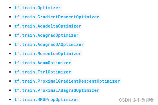
TensorFlow2 study notes: 7. Optimizer
Copy攻城狮5分钟在线体验 MindIR 格式模型生成

【Copy攻城狮日志】飞浆学院强化学习7日打卡营-学习笔记
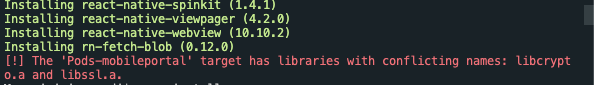
target has libraries with conflicting names: libcrypto.a and libssl.a.
随机推荐
深度学习理论——过拟合、欠拟合、正则化、优化器
MNIST手写数字识别 —— 从感知机到卷积神经网络
MNIST手写数字识别 —— 图像分析法实现二分类
WARNING: sql version 9.2, server version 11.0. Some psql features might not work.
Comparison of oracle's number and postgresql's numeric
0, deep learning 21 days learning challenge 】 【 set up learning environment
图像形变(插值方法)
[CV-Learning] Linear Classifier (SVM Basics)
Polynomial Regression (PolynomialFeatures)
动手学深度学习_softmax回归
MFC读取点云,只能正常显示第一个,显示后面时报错
lstm pipeline 过程理解(输入输出)
TensorFlow2 study notes: 8. tf.keras implements linear regression, Income dataset: years of education and income dataset
软著撰写注意事项
如何成长为高级工程师?
强化学习中,Q-Learning与Sarsa的差别有多大?
动手学深度学习_卷积神经网络CNN
TensorFlow2学习笔记:6、过拟合和欠拟合,及其缓解方案
机器学习——分类问题对于文字标签的处理(特征工程)
TensorFlow2 study notes: 5. Common activation functions