Paper notes: graph neural network gat

Abstract : Share your understanding of the paper . See the original Petar Velickovic, Guillem Cucurull, Arantxa Casanova, Adriana Romero, Pietro Lio, Yoshua Bengio, Graph attention networks, ICLR 2018, 1–12. Can be in ArXiv: 1710.10903v3 download . It's completely difficult to estimate the influence !

1. Contribution of thesis

• Overcome the shortcomings of the existing methods of graph convolution .
• No time-consuming matrix operation ( Such as inverse ).
• There is no need to predict the structure of the graph .
• Applicable to inductive and deductive problems .

2. Basic ideas

Use neighbor information , Map the original attributes of the nodes in the graph to a new space , To support later learning tasks .
This idea may be common to different graph Neural Networks .

3. programme

Table 1. Notations.

Symbol	meaning	remarks
$N$	Number of nodes
$F$	Original feature number
$F^{\prime }$	Original feature number	In the example 4
$\mathbf{h}$	Node feature set	$\{{\overrightarrow{h}}_1,\dots ,{\overrightarrow{h}}_N\}$
${\overrightarrow{h}}_i$	The first $i$ Characteristics of nodes	Belong to space ${\mathbb{R}}^F$
${\mathbf{h}}^{\prime }$	Node new feature set	$\{{\overrightarrow{h}}_1^{\prime },\dots ,{\overrightarrow{h}}_N^{\prime }\}$
${\overrightarrow{h}}_i^{\prime }$	The first $i$ New features of nodes	Belong to space ${\mathbb{R}}^{F^{\prime }}$
$\mathbf{W}$	Characteristic mapping matrix	Belong to ${\mathbb{R}}^{F\times F^{\prime }}$, All nodes share
${\mathcal{N}}_i$	node $i$ The neighborhood set of	Include $i$ own , In the example, the cardinality is 6
$\overrightarrow{\mathbf{a}}$	Feature weight vector	Belong to ${\mathbb{R}}^{2F^{\prime }}$, All nodes share , Corresponding to single-layer network
${\alpha }_{ij}$	node $j$ Yes $i$ Influence	The sum of the influences of all neighbor nodes is 1
${\overrightarrow{\alpha }}_{ij}$	node $j$ Yes $i$ Influence vector of	The length is $K$, Corresponding to the bull

Map node features to the new space , Using the attention mechanism $a$ Calculate the relationship between nodes
$$e_{ij}=a(\mathbf{W}{\overrightarrow{h}}_i,\mathbf{W}{\overrightarrow{h}}_j)\text{\hspace{1em}(1)}$$
Here only if $j$ yes $i$ When you are a neighbor on the network , Only calculated $e_{ij}$.
Carry it on softmax, Make nodes $i$ The corresponding weight sum is 1.
$${\alpha }_{ij}={\mathrm{s}\mathrm{o}\mathrm{f}\mathrm{t}\mathrm{m}\mathrm{a}\mathrm{x}}_j(e_{ij})=\frac{\exp (e_{ij})}{{\sum }_{k\in {\mathcal{N}}_i}\exp (e_{ik})}\text{\hspace{1em}(2)}$$
because $a$ The length will be $2F^{\prime }$ The column vector of is converted to a scalar , It can be written as a line vector of the same length ${\overrightarrow{\mathbf{a}}}^{\mathrm{T}}$. Plus an activation function , It can be realized with a single-layer neural network .

$${\alpha }_{ij}=\frac{\exp (\mathrm{L}\mathrm{e}\mathrm{a}\mathrm{k}\mathrm{y}\mathrm{R}\mathrm{e}\mathrm{L}\mathrm{u}({\overrightarrow{\mathbf{a}}}^{\mathrm{T}}[\mathbf{W}{\overrightarrow{h}}_i\Vert \mathbf{W}{\overrightarrow{h}}_j]))}{{\sum }_{k\in {\mathcal{N}}_i}\exp (\mathrm{L}\mathrm{e}\mathrm{a}\mathrm{k}\mathrm{y}\mathrm{R}\mathrm{e}\mathrm{L}\mathrm{u}({\overrightarrow{\mathbf{a}}}^{\mathrm{T}}[\mathbf{W}{\overrightarrow{h}}_i\Vert \mathbf{W}{\overrightarrow{h}}_k]))}\text{\hspace{1em}(2)}$$

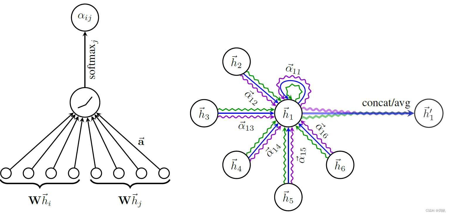
chart 1. GAT Core program . Left : $F^{\prime }=4$ When , from $\mathbf{W}$ The new space mapped to is 4 dimension . Corresponding $2F^{\prime }=8$ dimension . vector $\overrightarrow{\mathbf{a}}$ Shared by all nodes . Right : $K=3$ Head .

3.1 Scheme 1 : Single head

$${\overrightarrow{h}}_i^{\prime }=\sigma \left(\sum _{j\in i}{\alpha }_{ij}\mathbf{W}{\overrightarrow{h}}_j\right)\text{\hspace{1em}(4)}$$
All neighbor nodes are mapped to the new space first ( Such as 4 dimension ), Then the weighted sum is calculated according to its influence , And use sigmoid Isononlinear activation function , What you finally get is 4 Dimension vector .

3.2 Option two : Multi head connection

$${\overrightarrow{h}}_i^{\prime }={\Vert }_{k=1}^K\sigma \left(\sum _{j\in {\mathcal{N}}_i}{\alpha }_{ij}^k{\mathbf{W}}^k{\overrightarrow{h}}_j\right)\text{\hspace{1em}(5)}$$
$K$ Get the corresponding new vectors respectively , chart 1 The right shows 3 Head , So the last vector is $3\times 4=12$ dimension .

3.3 Option three : Long average

$${\overrightarrow{h}}_i^{\prime }=\sigma \left(\frac{1}{K}\sum _{k=1}^K\sum _{j\in {\mathcal{N}}_i}{\alpha }_{ij}^k{\mathbf{W}}^k{\overrightarrow{h}}_j\right)\text{\hspace{1em}(5)}$$
Just average , The last vector is $4$ dimension .

4. doubt

• problem : there $\mathbf{W}$ And $\overrightarrow{\mathbf{a}}$ How to learn ?
  guess : From related work , That is, the necessary knowledge is obtained in the graph neural network . This paper just wants to describe different core technologies .
  If the output of this network is used as the input of other networks ( The final output is class labels, etc ), It is possible to learn accordingly .
  Tang Wentao's explanation : In essence, it is equivalent to matrix multiplication ( Linear regression ), You can see from the code of the paper : In the training phase , The whole training set is entered ( Characteristic matrix and adjacency matrix of samples ), adopt $\mathbf{W}$ and $\overrightarrow{\mathbf{a}}$ Get the prediction label of the training set ( First, get the self attention weight of each sample for all samples , Then according to the adjacency matrix mask, Then normalize the weight as a layer of self attention ), Then proceed loss Calculation and dissemination of .

• problem : Why use when calculating influence LeakyReLU, When calculating the final eigenvector sigmoid?
  Force to explain : The former is only different from the latter ( It's not necessary ), The latter is to change linearity ( It is necessary to ).
  Tang Wentao's explanation : Calculate influence using LeakyReLU: Pay more attention to the neighbor nodes that are more positively related to the target node .
  The final eigenvector uses sigmoid It should be to prevent the value from being too large , Affect the next level of learning , Because the self attention mechanism is relatively unstable （ From my previous experiments ）, High requirements for the range and density of values （ Small scope :0-1 And so on , More dense ）.
  Besides , stay GAT The source code given in the paper can be seen , The author uses only two layers of self attention network for all data sets , also dropout All set to 0.5-0.8, It can be seen that it is easier to over fit .

5. Summary

• utilize $\mathbf{W}$ Linear mapping to new space .
• utilize $\overrightarrow{\mathbf{a}}$ Calculate the influence of each neighbor ${\alpha }_{ij}$. $\overrightarrow{\mathbf{a}}$ Only for the corresponding attribute , Not affected by neighbor number . ${\alpha }_{ij}$ The calculation of involves LeakyReLU Use of activation functions .
• Use bulls to increase stability .
• Calculating mean 、 Using nonlinear function activation will not change the dimension of the vector .