当前位置:网站首页>Attitude estimation (complementary filtering)
Attitude estimation (complementary filtering)
2022-07-07 22:16:00 【r1ch4rd】
Reference material :
A Complementary Filter for Attitude Estimation of a Fixed-Wing UAV
mahony Complementary filter
px4 Source code v1.7.3
Quaternion attitude solution
While looking at the program, talk about the principle :
AttitudeEstimatorQ::init()
The process of getting the initial quaternion :
1、 First built on NED Rotation matrix under system
k⃗ k → by z Axis , Direction is D towards , Vertical down
    // Rotation matrix can be easily constructed from acceleration and mag field vectors
    // 'k' is Earth Z axis (Down) unit vector in body frame

    Vector<3> k = -_accel;
k.normalize();i⃗ i → yes NED In a coordinate system x Axis , From Schmidt orthogonalization :
    //'i' is Earth X axis (North) unit vector in body frame, orthogonal with 'k'
    Vector<3> i = (_mag - k * (_mag * k));
    i.normalize();
Schmidt orthogonalization :
β2=α2−(α2,β1)(β1,β1)⋅β1 β 2 = α 2 − ( α 2 , β 1 ) ( β 1 , β 1 ) ⋅ β 1
k⃗ k → It has been normalized, so the denominator is 1
j⃗ j → yes NED In a coordinate system y Axis , from i⃗ i → ,k⃗ k → Cross multiply to get the vertical vector
    // 'j' is Earth Y axis (East) unit vector in body frame, orthogonal with 'k' and 'i'
    Vector<3> j = k % i;
2、 Fill the rotation matrix , And convert to quaternion :
    // Fill rotation matrix
    Matrix<3, 3> R;
    R.set_row(0, i);
    R.set_row(1, j);
    R.set_row(2, k);

    // Convert to quaternion
    _q.from_dcm(R)
Four yuan number Q Q And rotation matrix The transformation of
⎧⎩⎨⎪⎪⎪⎪⎪⎪⎪⎪⎪⎪⎪⎪⎪⎪q0=12(1+r11+r22+r33)−−−−−−−−−−−−−−−−√q1=14q0(r32−r23)q2=14q0(r31−r13)q3=14q0(r21−r12)⎫⎭⎬⎪⎪⎪⎪⎪⎪⎪⎪⎪⎪⎪⎪⎪⎪ { q 0 = 1 2 ( 1 + r 11 + r 22 + r 33 ) q 1 = 1 4 q 0 ( r 32 − r 23 ) q 2 = 1 4 q 0 ( r 31 − r 13 ) q 3 = 1 4 q 0 ( r 21 − r 12 ) }
3、 After correction according to magnetic declination , Normalize quaternions , Initialization complete .
// Compensate for magnetic declination
Quaternion decl_rotation;
decl_rotation.from_yaw(_mag_decl);
_q = decl_rotation * _q;

_q.normalize();
update(); Update quaternion
1、 Execute the initialization function once , Get the first quaternion
    if (!_inited) {

        if (!_data_good) {
            return false;
        }

        return init();
    }
2、px4 The means of calibration in includes vision , Motion capture , Magnetometer ; The first two belong to external heading information and will not be discussed , Only calibrate the magnetometer .
    if (_ext_hdg_mode == 0 || !_ext_hdg_good) {
        //  Magnetometer calibration
        //  Convert from volume coordinate system to navigation coordinate system
        Vector<3> mag_earth = _q.conjugate(_mag);

        float mag_err = _wrap_pi(atan2f(mag_earth(1), mag_earth(0)) - _mag_decl);// Make a difference with the automatically obtained magnetic declination
        float gainMult = 1.0f;
        const float fifty_dps = 0.873f;

        if (spinRate > fifty_dps) {
            gainMult = math::min(spinRate / fifty_dps, 10.0f);
        }

        // Project magnetometer correction to body frame
        corr += _q.conjugate_inversed(Vector<3>(0.0f, 0.0f, -mag_err)) * _w_mag * gainMult;
    }

    _q.normalize();
First, convert the magnetometer reading to the navigation coordinate system :
The output of the magnetometer is the angle between the current body and the geomagnetic field . The measuring principle is similar to that of a compass . Good low frequency characteristics , But it is easily disturbed by the surrounding magnetic field .
px4 of use GPS Information for calibration :
Convert the reading of magnetometer from vector to angle ; This angle is subtracted by GPS The magnetic bias obtained _mag_decl ; Get the magnetic field deviation mag_err;
float mag_err = _wrap_pi(atan2f(mag_earth(1), mag_earth(0)) - _mag_decl);
*arctan and arcsin The result is [−π2,π2] [ − π 2 , π 2 ] , This does not cover all orientations ( But for the θ θ The value range of angle has met ), So we need to use atan2f Instead of arctan, The value range becomes [−π,π] [ − π , π ] .
**_wrap_pi Yes, it will [0,2π] [ 0 , 2 π ] Mapping to [−π,π] [ − π , π ] On .
take mag_err Convert to the body coordinate system , And multiply by the weight
_q.normalize(); Quaternion normalization , The normalization here is used for correction update_mag_declination Deviation after . 3、 Accelerometer calibration
    Vector<3> k(
        2.0f * (_q(1) * _q(3) - _q(0) * _q(2)),
        2.0f * (_q(2) * _q(3) + _q(0) * _q(1)),
        (_q(0) * _q(0) - _q(1) * _q(1) - _q(2) * _q(2) + _q(3) * _q(3))
    );
k k Represents the vector of gravity vector in the body coordinate system :
eacc e a c c By Δqacc Δ q a c c and k k Cross multiply to get ; It is obtained by the accelerometer through low-pass filtering .
corr += (k % (_accel - _pos_acc).normalized()) * _w_accel;
_accel Is the accelerometer reading ;
_pos_acc Is estimated by location (GPS) The acceleration obtained by differentiation ;
_accel - _pos_acc Represents the acceleration vector of the aircraft minus its horizontal component ;
k And (_accel - _pos_acc) Cross riding , Get deviation ;
Program so far ,corr=eacc+emag c o r r = e a c c + e m a g
4、 Correct the gyroscope
    // Gyro bias estimation
    if (spinRate < 0.175f) {
        _gyro_bias += corr * (_w_gyro_bias * dt);// The correction value here is  mahony  Filtered  pi  Controller   Integral part ;

        // Gyro deviation upper limit
        for (int i = 0; i < 3; i++) {
            _gyro_bias(i) = math::constrain(_gyro_bias(i), -_bias_max, _bias_max);
        }

    }
5、_gyro_bias Over time , Non return to zero
_rates = _gyro + _gyro_bias;
corr += _rates;
PI The control of the P term ,corr=_rates+corr+ki∫corrdt c o r r = _ r a t e s + c o r r + k i ∫ c o r r d t
At this time corr c o r r Angular velocity obtained for final calibration
_q += _q.derivative(corr) * dt;
6、 First order Runge Kutta derivation :
ω=corr ω = c o r r
So we get quaternion update matrix :
    // Check whether quaternions diverge , If it is divergent, use the last updated q

    if (!(PX4_ISFINITE(_q(0)) && PX4_ISFINITE(_q(1)) &&
          PX4_ISFINITE(_q(2)) && PX4_ISFINITE(_q(3)))) {

        _q = q_last;
        _rates.zero();
        _gyro_bias.zero();
        return false;
}边栏推荐
- Restapi version control strategy [eolink translation]
- Pdf document signature Guide
- Jerry's key to initiate pairing [chapter]
- Node:504 error reporting
- [开源] .Net ORM 访问 Firebird 数据库
- Crawler (17) - Interview (2) | crawler interview question bank
- Kirin Xin'an operating system derivative solution | storage multipath management system, effectively improving the reliability of data transmission
- Ternary expressions, generative expressions, anonymous functions
- Leetcode SQL first day
- How to turn on win11 game mode? How to turn on game mode in win11
猜你喜欢
谈谈制造企业如何制定敏捷的数字化转型策略

How to quickly check whether the opening area ratio of steel mesh conforms to ipc7525

An overview of the latest research progress of "efficient deep segmentation of labels" at Shanghai Jiaotong University, which comprehensively expounds the deep segmentation methods of unsupervised, ro
Where is the big data open source project, one-stop fully automated full life cycle operation and maintenance steward Chengying (background)?
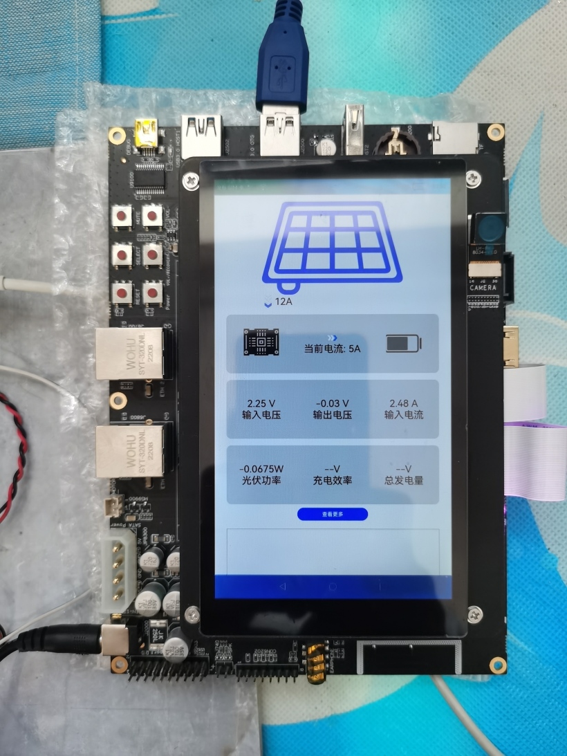
#DAYU200体验官#MPPT光伏发电项目 DAYU200、Hi3861、华为云IotDA
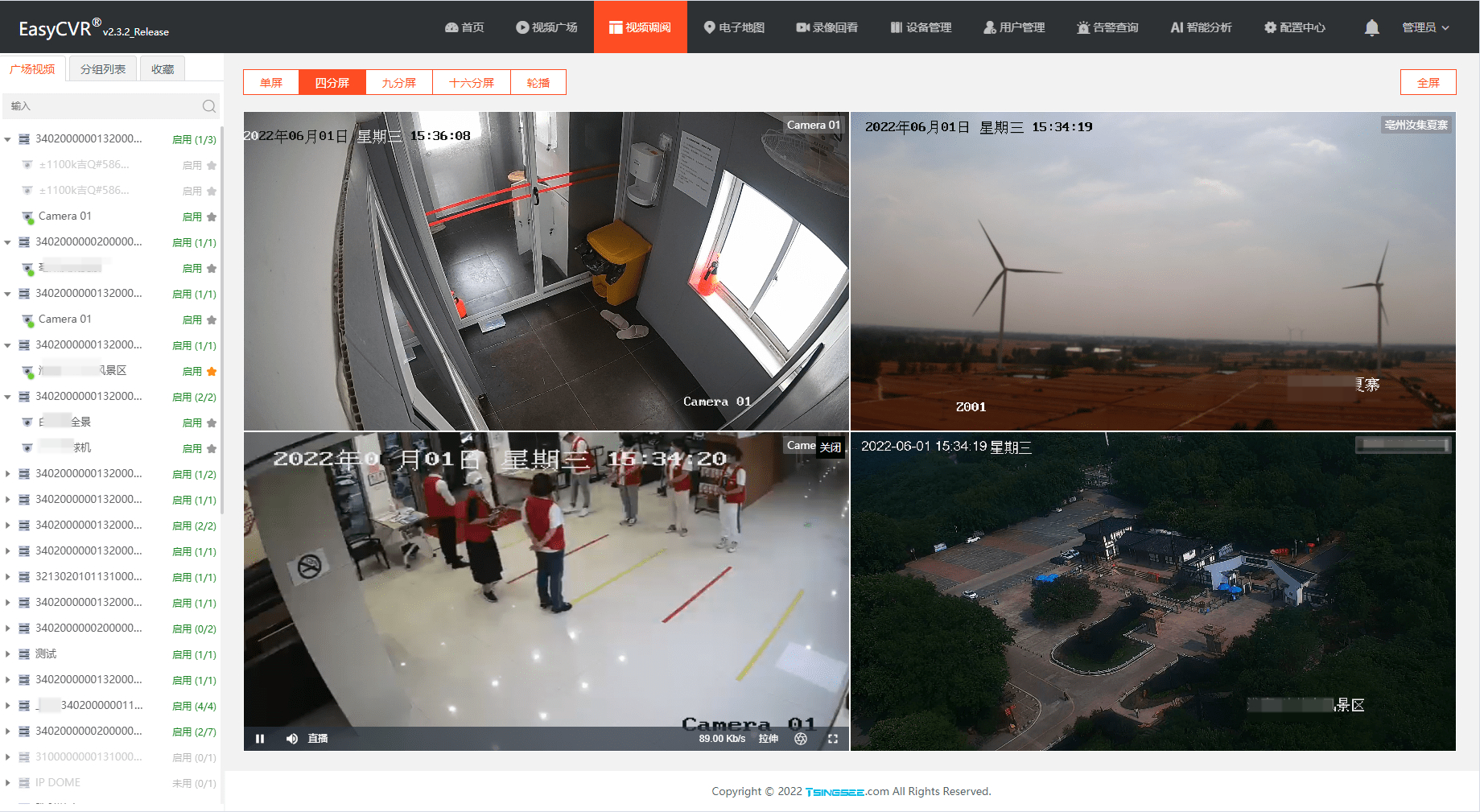
NVR硬盤錄像機通過國標GB28181協議接入EasyCVR,設備通道信息不顯示是什麼原因?

Index summary (assault version)
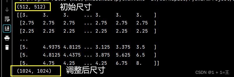
Cv2.resize function reports an error: error: (-215:assertion failed) func= 0 in function ‘cv::hal::resize‘
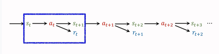
强化学习-学习笔记9 | Multi-Step-TD-Target
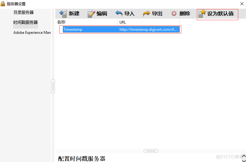
Pdf document signature Guide
随机推荐
反爬通杀神器
The essence of analog Servlet
Overseas agent recommendation
Jerry's test box configuration channel [chapter]
Leetcode SQL first day
An in-depth understanding of fp/fn/precision/recall
应用实践 | 数仓体系效率全面提升!同程数科基于 Apache Doris 的数据仓库建设
为什么Win11不能显示秒数?Win11时间不显示秒怎么解决?
Win11如何解禁键盘?Win11解禁键盘的方法
Ant destination multiple selection
Navicat connect 2002 - can't connect to local MySQL server through socket '/var/lib/mysql/mysql Sock 'solve
Relationship between URL and URI
Jerry's about TWS channel configuration [chapter]
Song list 11111
Application practice | the efficiency of the data warehouse system has been comprehensively improved! Data warehouse construction based on Apache Doris in Tongcheng digital Department
NVR硬盘录像机通过国标GB28181协议接入EasyCVR,设备通道信息不显示是什么原因?
Jerry's manual matching method [chapter]
23. Merge K ascending linked lists -c language
npm uninstall和rm直接删除的区别
Oracle advanced (VI) Oracle expdp/impdp details