当前位置:网站首页>Bidirectional RNN and stacked bidirectional RNN
Bidirectional RNN and stacked bidirectional RNN
2022-07-05 10:49:00 【Don't wait for shy brother to develop】
two-way RNN Two way with stacking RNN
1、 two-way RNN
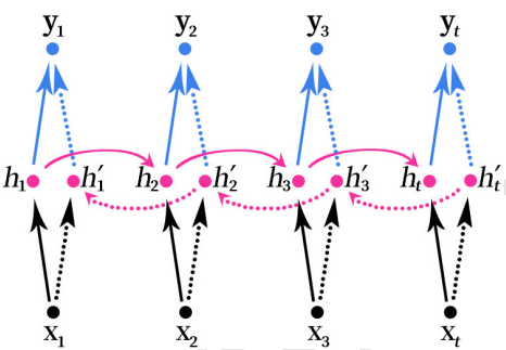
two-way RNN(Bidirectional RNN) The structure of is shown in the figure below .
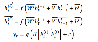
h t → = f ( W → x t + V → h t − 1 → + b → ) h t ← = f ( W ← x t + V ← h t − 1 ← + b ← ) y t = g ( U [ h t → ; h t ← ] + c ) \overrightarrow{h_t}=f(\overrightarrow{W}x_t+\overrightarrow{V}\overrightarrow{h_{t-1}}+\overrightarrow{b})\\ \overleftarrow{h_t}=f(\overleftarrow{W}x_t+\overleftarrow{V}\overleftarrow{h_{t-1}}+\overleftarrow{b})\\ y_t=g(U[\overrightarrow{h_t};\overleftarrow{h_t}]+c) ht=f(Wxt+Vht−1+b)ht=f(Wxt+Vht−1+b)yt=g(U[ht;ht]+c)
there RNN You can use either RNN structure SimpleRNN,LSTM or GRU. Here, the arrow indicates propagation from left to right or from right to left , Prediction for each moment , Both require feature vectors from both directions , Splicing (Concatenate) Then predict the results . Although the arrows are different , But the parameters are the same set . Some models also Two different sets of parameters can be used .f,g Is the activation function , [ h t → ; h t ← ] [\overrightarrow{h_t};\overleftarrow{h_t}] [ht;ht] Represents data splicing (Concatenate).
Bidirectional RNN At the same time “ In the past ” and “ future ” Information about . The above figure shows a sequence with a length of 4 Two way RNN structure .
Such as input x 1 x_1 x1 Transmit to the hidden layer along the solid arrow to get h 1 h_1 h1, Then it needs to be reused x t x_t xt To calculate the h t ′ h_t' ht′, utilize x 3 x_3 x3 and h t ′ h_t' ht′ To calculate the h 3 ′ h_3' h3′, utilize x 2 x_2 x2 and h 3 ′ h_3' h3′ To calculate the h 2 ′ h_2' h2′, utilize x 1 x_1 x1 and ’h_2’ To calculate the h 1 ′ h_1' h1′, Finally, put h 1 h_1 h1 and h 1 ′ h_1' h1′ Data stitching (Concatenate), Get the output y 1 y_1 y1. And so on , At the same time, the forward and reverse transfer data are used to predict the results .
two-way RNN It's like reading an article from the beginning to the end when we do reading comprehension , Then read the article again from the back , Then do the question . It is possible to have a new and different understanding when reading the article again from the back to the front , Finally, the model may get better results .
2、 Stacked two-way RNN
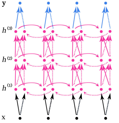
Stacked two-way RNN(Stacked Bidirectional RNN) Its structure is shown in the figure above . The picture above is a stack 3 A hidden layer RNN The Internet .
Be careful , The stacking here is bidirectional RNN There is not only two-way RNN Can be stacked , Actually arbitrary RNN Can be stacked , Such as SimpleRNN、LSTM and GRU These recurrent neural networks can also be stacked .
Stacking means in RNN Multiple layers are superimposed in the structure of , Be similar to BP Multiple layers can be superimposed in Neural Networks , Increase the nonlinearity of the network .
3、 two-way LSTM Realization MNIST Data set classification
import tensorflow as tf
from tensorflow.keras.models import Sequential
from tensorflow.keras.layers import Dense
from tensorflow.keras.layers import LSTM,Dropout,Bidirectional
from tensorflow.keras.optimizers import Adam
import matplotlib.pyplot as plt
# Loading data sets
mnist = tf.keras.datasets.mnist
# Load data , The training set and test set have been divided when the data is loaded
# Training set data x_train The data shape of is (60000,28,28)
# Training set label y_train The data shape of is (60000)
# Test set data x_test The data shape of is (10000,28,28)
# Test set label y_test The data shape of is (10000)
(x_train, y_train), (x_test, y_test) = mnist.load_data()
# Normalize the data of training set and test set , It helps to improve the training speed of the model
x_train, x_test = x_train / 255.0, x_test / 255.0
# Turn the labels of training set and test set into single hot code
y_train = tf.keras.utils.to_categorical(y_train,num_classes=10)
y_test = tf.keras.utils.to_categorical(y_test,num_classes=10)
# data size - The line has 28 Pixel
input_size = 28
# Sequence length - Altogether 28 That's ok
time_steps = 28
# Hidden layer memory block Number
cell_size = 50
# Creating models
# The data input of the recurrent neural network must be 3 D data
# The data format is ( Number of data , Sequence length , data size )
# Loaded mnist The format of the data just meets the requirements
# Notice the input_shape There is no need to set the quantity of data when setting the model data input
model = Sequential([
Bidirectional(LSTM(units=cell_size,input_shape=(time_steps,input_size),return_sequences=True)),
Dropout(0.2),
Bidirectional(LSTM(cell_size)),
Dropout(0.2),
# 50 individual memory block Output 50 Value and output layer 10 Neurons are fully connected
Dense(10,activation=tf.keras.activations.softmax)
])
# The data input of the recurrent neural network must be 3 D data
# The data format is ( Number of data , Sequence length , data size )
# Loaded mnist The format of the data just meets the requirements
# Notice the input_shape There is no need to set the quantity of data when setting the model data input
# model.add(LSTM(
# units = cell_size,
# input_shape = (time_steps,input_size),
# ))
# 50 individual memory block Output 50 Value and output layer 10 Neurons are fully connected
# model.add(Dense(10,activation='softmax'))
# Define optimizer
adam = Adam(lr=1e-3)
# Define optimizer ,loss function, The accuracy of calculation during training Using the cross entropy loss function
model.compile(optimizer=adam,loss='categorical_crossentropy',metrics=['accuracy'])
# Training models
history=model.fit(x_train,y_train,batch_size=64,epochs=10,validation_data=(x_test,y_test))
# Print model summary
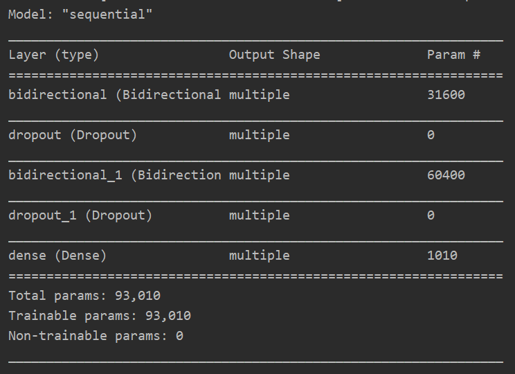
model.summary()
loss=history.history['loss']
val_loss=history.history['val_loss']
accuracy=history.history['accuracy']
val_accuracy=history.history['val_accuracy']
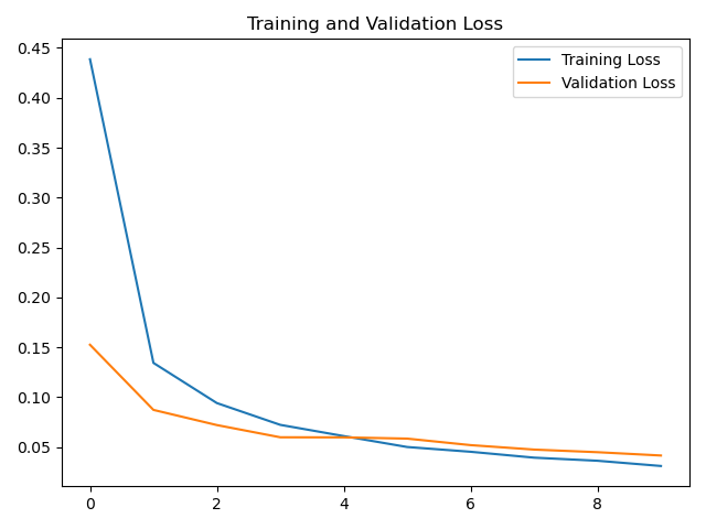
# draw loss curve
plt.plot(loss, label='Training Loss')
plt.plot(val_loss, label='Validation Loss')
plt.title('Training and Validation Loss')
plt.legend()
plt.show()
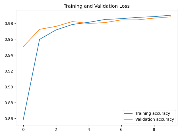
# draw acc curve
plt.plot(accuracy, label='Training accuracy')
plt.plot(val_accuracy, label='Validation accuracy')
plt.title('Training and Validation Loss')
plt.legend()
plt.show()
This may be easier to deal with text data , It's a little reluctant to use this model here , Just a simple test .
Model summary :
acc curve :
loss curve :

边栏推荐
- PWA (Progressive Web App)
- 2022年流动式起重机司机考试题库及模拟考试
- Web3基金会「Grant计划」赋能开发者,盘点四大成功项目
- 2021年山东省赛题库题目抓包
- Common functions of go-2-vim IDE
- Cross page communication
- Array
- In the year of "mutual entanglement" of mobile phone manufacturers, the "machine sea tactics" failed, and the "slow pace" playing method rose
- 第五届 Polkadot Hackathon 创业大赛全程回顾,获胜项目揭秘!
- [JS] array dimensionality reduction
猜你喜欢
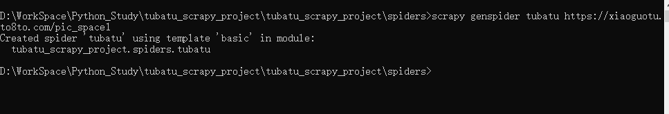
爬虫(9) - Scrapy框架(1) | Scrapy 异步网络爬虫框架
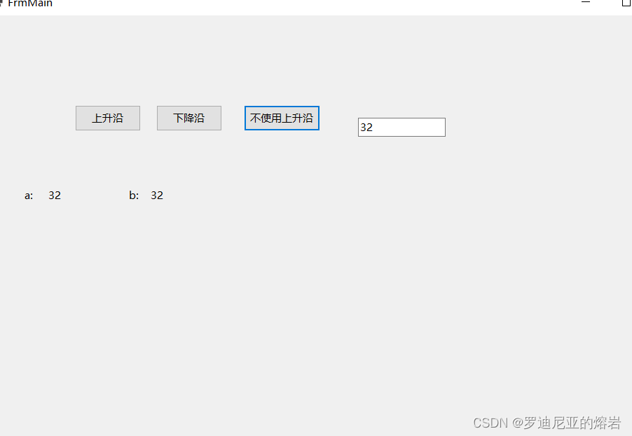
Implement the rising edge in C #, and simulate the PLC environment to verify the difference between if statement using the rising edge and not using the rising edge
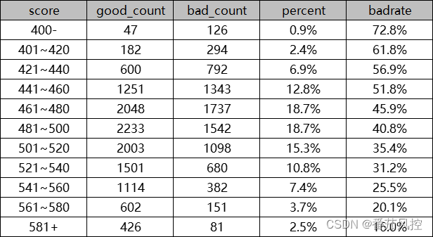
风控模型启用前的最后一道工序,80%的童鞋在这都踩坑
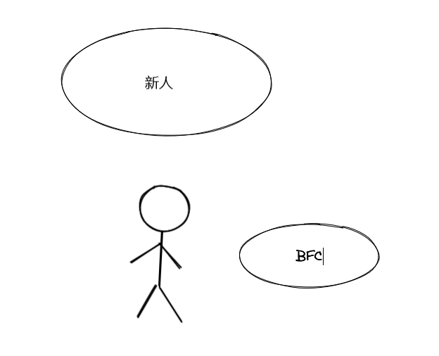
【js学习笔记五十四】BFC方式
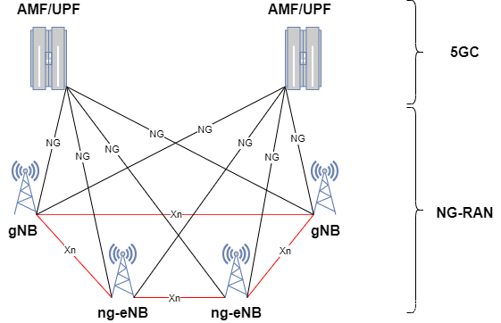
5g NR system architecture
![[observation] with the rise of the](/img/9a/8bbf98e6aed80638f4340aacec2ea9.jpg)
[observation] with the rise of the "independent station" model of cross-border e-commerce, how to seize the next dividend explosion era?

Pseudo class elements -- before and after

Go-3-the first go program

Review the whole process of the 5th Polkadot Hackathon entrepreneurship competition, and uncover the secrets of the winning projects!

Based on shengteng AI Yisa technology, it launched a full target structured solution for video images, reaching the industry-leading level
随机推荐
Solution to the length of flex4 and Flex3 combox drop-down box
Nine degrees 1480: maximum ascending subsequence sum (dynamic programming idea for the maximum value)
跨页面通讯
Go项目实战—参数绑定,类型转换
How can gbase 8C database view the login information of the login user, such as the date, time and IP of the last login authentication?
Implement the rising edge in C #, and simulate the PLC environment to verify the difference between if statement using the rising edge and not using the rising edge
2022年T电梯修理操作证考试题及答案
【Vite】1371- 手把手开发 Vite 插件
Based on shengteng AI Yisa technology, it launched a full target structured solution for video images, reaching the industry-leading level
Based on shengteng AI Aibi intelligence, we launched a digital solution for bank outlets to achieve full digital coverage of information from headquarters to outlets
关于vray 5.2的使用(自研笔记)(二)
关于vray5.2怎么关闭日志窗口
风控模型启用前的最后一道工序,80%的童鞋在这都踩坑
Customize the left sliding button in the line in the applet, which is similar to the QQ and Wx message interface
websocket
微信核酸检测预约小程序系统毕业设计毕设(7)中期检查报告
重磅:国产IDE发布,由阿里研发,完全开源!
Array
【DNS】“Can‘t resolve host“ as non-root user, but works fine as root
flex4 和 flex3 combox 下拉框长度的解决办法