当前位置:网站首页>Exploratory data analysis of heartbeat signal
Exploratory data analysis of heartbeat signal
2022-07-07 23:06:00 【Anny Linlin】
One 、 understand EDA
First, what is exploratory data analysis ? And the purpose of exploratory data analysis ?
Exploratory data analysis refers to the analysis of existing data ( Especially raw data from investigation or observation ) Explore with as few prior assumptions as possible , By drawing 、 Tabulation 、 Equation fitting 、 A data analysis method to explore the structure and law of data by calculating characteristic quantity . Guide data science practitioners in data processing and Feature Engineering steps , Make the structure and feature set of data set more reliable for the next prediction problem . It is worth noting that , EDA The process is the characteristics of the original data ( Statistical characteristics 、 Distribution characteristics 、 Correlation, etc ) Mining , But no features are deleted or constructed .
What kind of process is exploratory data analysis ?
1、 Load data science and visualization libraries :
Data Science Database pandas、numpy、scipy;
Visualization Library matplotlib、seabon;
2、 Loading data sets :
Training data and test data , Simple data observation , In general use head and shape.3、 Data overview :
adopt describe() To get familiar with the relevant statistics of data ; adopt info() To get familiar with data types .
4、 Judge whether the data is missing or abnormal
Check the existence of each column nan situation ; Outlier detection .
5、 Understand the distribution of predicted values
General distribution ( Unbounded Johnson distribution, etc ); see skewness and kurtosis; Look at the frequency of the predicted value .
Two 、 Use EDA
1、 Import library
import warnings
warnings.filterwarnings('ignore')
import missingno as msno
import pandas as pd
import matplotlib.pyplot as plt
import seaborn as sns
import numpy as np
2、 Loading data sets
train_data = pd.read_csv('train.csv')
test_data = pd.read_csv('testA.csv')
train_data.head().append(train_data.tail())
train_data.shape
3、 Data overview
train_data.describe()
train_data.info
4、 Judge the missing value and abnormal data
train_data.isnull().sum()
5、 Understand the distribution of predicted values
train_data['label']
train_data['label'].value_counts()
(1) General distribution :
import scipy.stats as st
y = train_data['label']
plt.subplot(121)
sns.distplot(y,rug=True,bins=20)
plt.subplot(122)
sns.distplot(y,kde=False,fit=st.norm)
plt.subplot(123)
sns.distplot(y,kde=False,fit=st.lognorm)
plt.show()
(2) see skewness and kurtosis
sns.distplot(train_data['label']);
print("Skewness: %f" % train_data['label'].skew())
print("Kurtosis: %f" % train_data['label'].kurt())
train_data.skew(),train_data.kurt()
(3) Look at the frequency of the predicted value
# View the specific frequency of prediction
plt.hist(train_data['label'],orientation='vertical',histtype='bar',color='red')
plt.show()
边栏推荐
- Cascade-LSTM: A Tree-Structured Neural Classifier for Detecting Misinformation Cascades-KDD2020
- Leetcode1984. Minimum difference in student scores
- One question per day - pat grade B 1002 questions
- 安踏DTC | 安踏转型,构建不只有FILA的增长飞轮
- De la famille debezium: SET ROLE statements supportant mysql8
- Why is network i/o blocked?
- What is fake sharing after filling the previous hole?
- [record of question brushing] 3 Longest substring without duplicate characters
- Software test classification
- 30讲 线性代数 第五讲 特征值与特征向量
猜你喜欢

Yarn cannot view the historical task log of yarn after enabling ACL user authentication. Solution
ASP.NET Core入门五
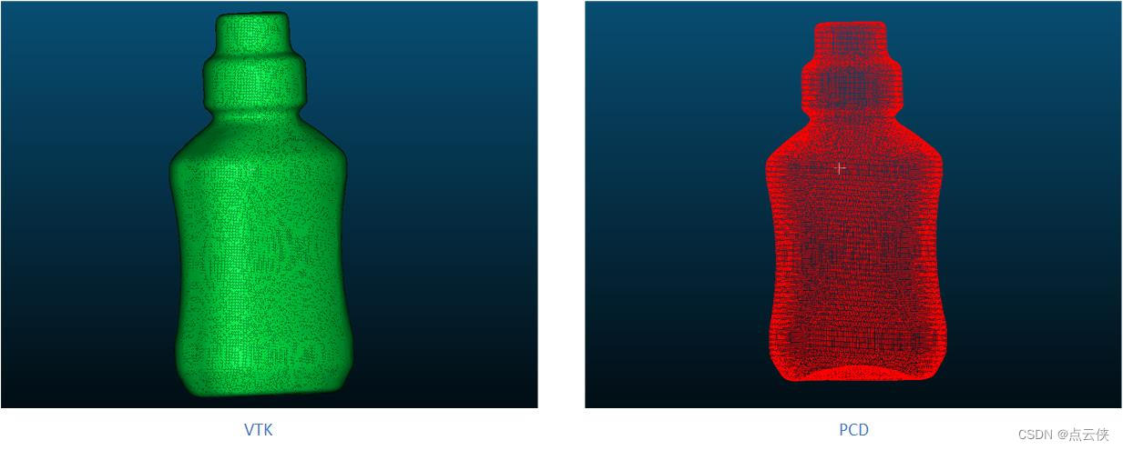
PCL . VTK files and Mutual conversion of PCD

0-5VAC转4-20mA交流电流隔离变送器/转换模块

Microbial Health Network, How to restore Microbial Communities

GBU1510-ASEMI电源专用15A整流桥GBU1510

Early childhood education industry of "screwing bar": trillion market, difficult to be a giant

行測-圖形推理-4-字母類
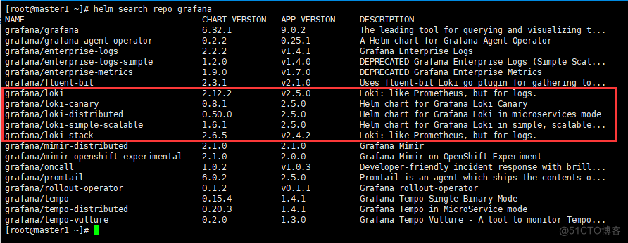
「开源摘星计划」Loki实现Harbor日志的高效管理

Comparison of various development methods of applets - cross end? Low code? Native? Or cloud development?
随机推荐
聊聊 Dart 的空安全 (null safety) 特性
Signal feature extraction +lstm to realize gear reducer fault diagnosis -matlab code
There is another problem just online... Warm
软件测评中心▏自动化测试有哪些基本流程和注意事项?
定位到最底部[通俗易懂]
Line test - graphic reasoning - 6 - similar graphic classes
Unity local coordinates and world coordinates
消费品企业敏捷创新转型案例
This time, let's clear up: synchronous, asynchronous, blocking, non blocking
Line test - graphic reasoning -5- one stroke class
Micro service remote debug, nocalhost + rainbow micro service development second bullet
Class implementation of linear stack and linear queue (another binary tree pointer version)
Line test graph reasoning graph group class
Sword finger offer 28 Symmetric binary tree
双非大厂测试员亲述:对测试员来说,学历重要吗?
Personal statement of testers from Shuangfei large factory: is education important for testers?
微服務遠程Debug,Nocalhost + Rainbond微服務開發第二彈
Debezium系列之: 支持在 KILL 命令中使用变量
Txt file virus
肠道里的微生物和皮肤上的一样吗?