当前位置:网站首页>Pytorch builds neural network to predict temperature
Pytorch builds neural network to predict temperature
2022-07-07 05:42:00 【Magnetoelectricity】
import numpy as np
import pandas as pd
import matplotlib.pyplot as plt
import torch
import torch.optim as optim
import warnings
warnings.filterwarnings("ignore")
%matplotlib inline
features = pd.read_csv('temps.csv')
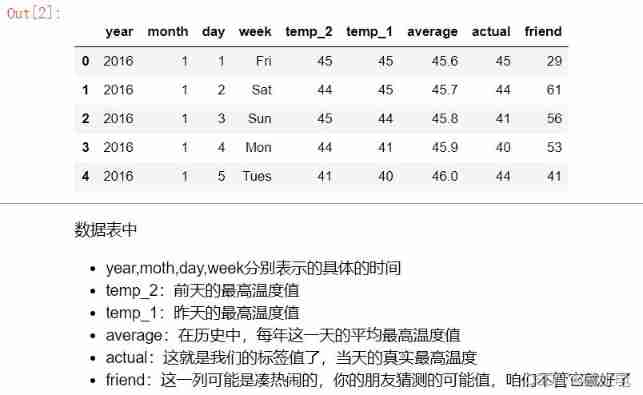
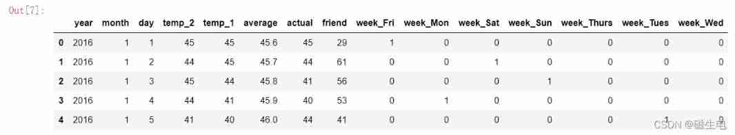
# See what the data looks like
features.head()
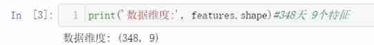
# Processing time data : Convert all time columns into datetime Format , Convenient visual display
import datetime
# Get years respectively , month , Japan
years = features['year']
months = features['month']
days = features['day']
# datetime Format
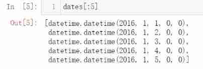
dates = [str(int(year)) + '-' + str(int(month)) + '-' + str(int(day)) for year, month, day in zip(years, months, days)]
dates = [datetime.datetime.strptime(date, '%Y-%m-%d') for date in dates]
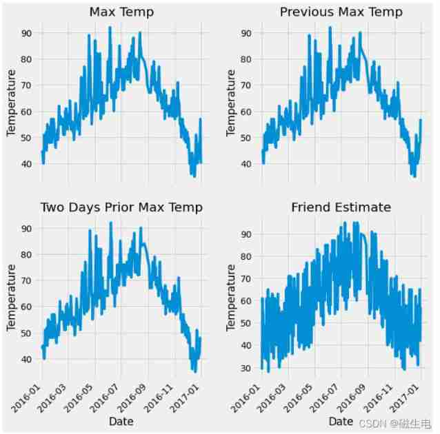
#  Prepare to draw
#  Specify the default style
plt.style.use('fivethirtyeight')

#  Setting up layout
fig, ((ax1, ax2), (ax3, ax4)) = plt.subplots(nrows=2, ncols=2, figsize = (10,10))
fig.autofmt_xdate(rotation = 45)

#  Label value
ax1.plot(dates, features['actual'])
ax1.set_xlabel(''); ax1.set_ylabel('Temperature'); ax1.set_title('Max Temp')

#  yesterday
ax2.plot(dates, features['temp_1'])
ax2.set_xlabel(''); ax2.set_ylabel('Temperature'); ax2.set_title('Previous Max Temp')

#  The day before yesterday
ax3.plot(dates, features['temp_2'])
ax3.set_xlabel('Date'); ax3.set_ylabel('Temperature'); ax3.set_title('Two Days Prior Max Temp')

#  My funny friend
ax4.plot(dates, features['friend'])
ax4.set_xlabel('Date'); ax4.set_ylabel('Temperature'); ax4.set_title('Friend Estimate')

plt.tight_layout(pad=2)
#  Hot coding alone   Right week 1 Code on Sunday   Convert all data into numerical form
features = pd.get_dummies(features)# Send the whole data in pd.get_dummies It will automatically judge which column is a string and can be encoded
features.head(5)
#  Specify the label to be trained before the training model X Y
labels = np.array(features['actual'])# take y value

#  Remove labels from features
features= features.drop('actual', axis = 1)# take x value

#  Save the names separately , For visual display
feature_list = list(features.columns)

#  Convert to appropriate format
features = np.array(features)
from sklearn import preprocessing
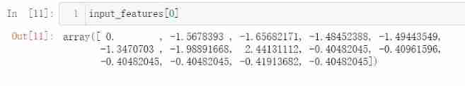
input_features = preprocessing.StandardScaler().fit_transform(features)# The data value difference between some columns is relatively large, and data standardization is needed for preprocessing , The convergence speed is faster after standardization , The loss value is smaller
torch Build a network model
# First of all, x y Turn into tensor The format of
x = torch.tensor(input_features, dtype = float)
y = torch.tensor(labels, dtype = float)
# Weight parameter initialization
weights = torch.randn((14, 128), dtype = float, requires_grad = True) # Cryptic layer 128 Neurons , The input layer passes through the hidden layer to get 128 Features
biases = torch.randn(128, dtype = float, requires_grad = True)
weights2 = torch.randn((128, 1), dtype = float, requires_grad = True) # Because it's a return mission , So finally, we need to get a value to represent w, So we need to go through a full connection layer [128,1]
biases2 = torch.randn(1, dtype = float, requires_grad = True)
learning_rate = 0.001
losses = []
for i in range(1000):
# Calculate hidden layer
hidden = x.mm(weights) + biases#[348,14] *[14,128] x.mm() Representation matrix multiplication
# Add activation function
hidden = torch.relu(hidden)
# Predicted results
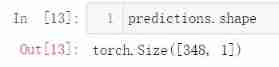
predictions = hidden.mm(weights2) + biases2
# Calculate the loss by
loss = torch.mean((predictions - y) ** 2)
losses.append(loss.data.numpy())
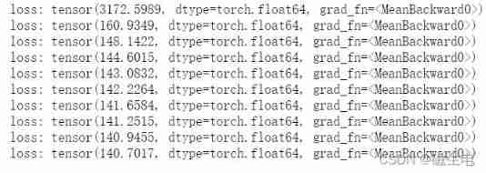
# Print loss value
if i % 100 == 0:
print('loss:', loss)
# Backward propagation calculation
loss.backward()
# Update parameters
weights.data.add_(- learning_rate * weights.grad.data) # The minus sign means the gradient drops
biases.data.add_(- learning_rate * biases.grad.data)
weights2.data.add_(- learning_rate * weights2.grad.data)
biases2.data.add_(- learning_rate * biases2.grad.data)
# Remember to empty every iteration
weights.grad.data.zero_()
biases.grad.data.zero_()
weights2.grad.data.zero_()
biases2.grad.data.zero_()
It's simpler to build a network model
The first is to calculate all the input data together , Next use miniBatch Small batch calculation
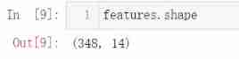
input_size = input_features.shape[1]
hidden_size = 128
output_size = 1
batch_size = 16
# Here, the network architecture is built in advance
my_nn = torch.nn.Sequential(
    torch.nn.Linear(input_size, hidden_size),
    torch.nn.Sigmoid(),
    torch.nn.Linear(hidden_size, output_size),
)
cost = torch.nn.MSELoss(reduction='mean')
optimizer = torch.optim.Adam(my_nn.parameters(), lr = 0.001)# The simple method replaces the previous need for handwriting gradient descent and gradient update   The loss function is also called directly MSE Just lose
# The optimizer uses ADam The learning rate can be adjusted dynamically , Adding attenuation function makes the learning rate slowly decrease as the iteration proceeds
#  Training network
losses = []
for i in range(1000):
    batch_loss = []
    # MINI-Batch Methods to train
    for start in range(0, len(input_features), batch_size):
        end = start + batch_size if start + batch_size < len(input_features) else len(input_features)
        xx = torch.tensor(input_features[start:end], dtype = torch.float, requires_grad = True)
        yy = torch.tensor(labels[start:end], dtype = torch.float, requires_grad = True)
        prediction = my_nn(xx)# Forward propagation prediction
        loss = cost(prediction, yy)# Calculate the loss
        optimizer.zero_grad()# Gradient clear
        loss.backward(retain_graph=True)# Back propagation
        optimizer.step()# Gradient update
        batch_loss.append(loss.data.numpy())

    #  Print loss
    if i % 100==0:
        losses.append(np.mean(batch_loss))
        print(i, np.mean(batch_loss))
Predict training results
x = torch.tensor(input_features, dtype = torch.float)
predict = my_nn(x).data.numpy()# Turn into numpy1 Grid is convenient for drawing
#  Convert date format
dates = [str(int(year)) + '-' + str(int(month)) + '-' + str(int(day)) for year, month, day in zip(years, months, days)]
dates = [datetime.datetime.strptime(date, '%Y-%m-%d') for date in dates]

#  Create a table to store dates and their corresponding tag values
true_data = pd.DataFrame(data = {
    'date': dates, 'actual': labels})

#  Empathy , Create another one to save the date and its corresponding model prediction value
months = features[:, feature_list.index('month')]
days = features[:, feature_list.index('day')]
years = features[:, feature_list.index('year')]

test_dates = [str(int(year)) + '-' + str(int(month)) + '-' + str(int(day)) for year, month, day in zip(years, months, days)]

test_dates = [datetime.datetime.strptime(date, '%Y-%m-%d') for date in test_dates]

predictions_data = pd.DataFrame(data = {
    'date': test_dates, 'prediction': predict.reshape(-1)}) #predict.reshape(-1) Means a column , Cannot be in matrix format
#  True value
plt.plot(true_data['date'], true_data['actual'], 'b-', label = 'actual')

#  Predictive value
plt.plot(predictions_data['date'], predictions_data['prediction'], 'ro', label = 'prediction')
plt.xticks(rotation = '60');
plt.legend()

#  Title
plt.xlabel('Date'); plt.ylabel('Maximum Temperature (F)'); plt.title('Actual and Predicted Values');
The experimental data set is transformed into .csv Files use
边栏推荐
- 淘寶商品詳情頁API接口、淘寶商品列錶API接口,淘寶商品銷量API接口,淘寶APP詳情API接口,淘寶詳情API接口
- LabVIEW is opening a new reference, indicating that the memory is full
- Leakage relay jelr-250fg
- The year of the tiger is coming. Come and make a wish. I heard that the wish will come true
- 毕业之后才知道的——知网查重原理以及降重举例
- Realize GDB remote debugging function between different network segments
- 删除文件时提示‘源文件名长度大于系统支持的长度’无法删除解决办法
- 一条 update 语句的生命经历
- 《2022中国低/无代码市场研究及选型评估报告》发布
- 【oracle】简单的日期时间的格式化与排序问题
猜你喜欢

English grammar_ Noun possessive
![[论文阅读] A Multi-branch Hybrid Transformer Network for Corneal Endothelial Cell Segmentation](/img/f6/cd307c03ea723e1fb6a0011b37d3ef.png)
[论文阅读] A Multi-branch Hybrid Transformer Network for Corneal Endothelial Cell Segmentation
1.AVL树:左右旋-bite
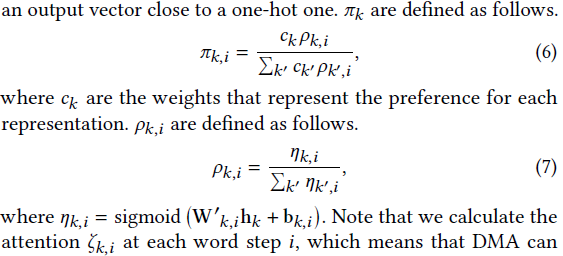
论文阅读【Sensor-Augmented Egocentric-Video Captioning with Dynamic Modal Attention】
什么是依赖注入(DI)
Reading the paper [sensor enlarged egocentric video captioning with dynamic modal attention]

K6el-100 leakage relay
Two person game based on bevy game engine and FPGA
![[JS component] date display.](/img/26/9bfc752c8c9a933a8e33b59e0488a2.jpg)
[JS component] date display.
Pinduoduo product details interface, pinduoduo product basic information, pinduoduo product attribute interface
随机推荐
Flink SQL realizes reading and writing redis and dynamically generates hset key
Realize GDB remote debugging function between different network segments
Message queuing: how to ensure that messages are not lost
Use Zhiyun reader to translate statistical genetics books
[binary tree] binary tree path finding
The navigation bar changes colors according to the route
Flinksql 读写pgsql
分布式事务介绍
Leakage relay llj-100fs
Design, configuration and points for attention of network arbitrary source multicast (ASM) simulation using OPNET
论文阅读【Semantic Tag Augmented XlanV Model for Video Captioning】
bat 批示处理详解
Web Authentication API兼容版本信息
When deleting a file, the prompt "the length of the source file name is greater than the length supported by the system" cannot be deleted. Solution
R语言【逻辑控制】【数学运算】
什么是依赖注入(DI)
Getting started with DES encryption
sql优化常用技巧及理解
Summary of the mean value theorem of higher numbers
What are the common message queues?