当前位置:网站首页>[secretly kill little partner pytorch20 days -day01- example of structured data modeling process]
[secretly kill little partner pytorch20 days -day01- example of structured data modeling process]
2022-07-06 08:17:00 【Can't write code】
Catalog
import os
import datetime

# Print time
def printbar():
    nowtime = datetime.datetime.now().strftime('%Y-%m-%d %H:%M:%S')
    print("\n"+"=========="*8 + "%s"%nowtime)

utilize datetime Modular now Function to get the current time and pass strftime Format the output
1. Prepare the data
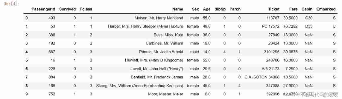
titanic The goal of the dataset is to predict, based on passenger information, that they are in Titanic Whether or not it can survive after hitting an iceberg .( Those who need data sets can pay more attention and contact me )
Structured data generally uses Pandas Medium DataFrame Pre treatment .
import numpy as np
import pandas as pd
import matplotlib.pyplot as plt
import torch
from torch import nn
from torch.utils.data import Dataset,DataLoader,TensorDataset

dftrain_raw = pd.read_csv('train.csv')
dftest_raw = pd.read_csv('test.csv')
dftrain_raw.head(10)
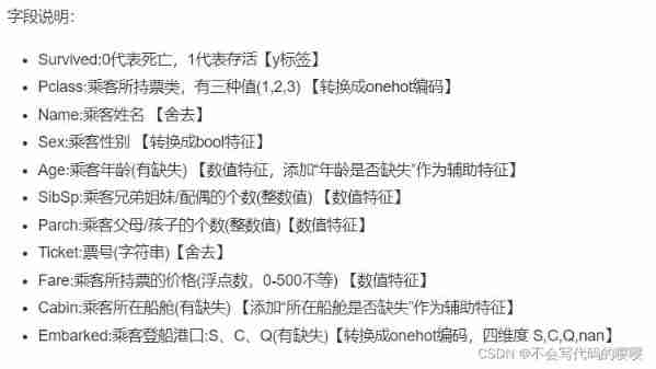
notes : there onehot Coding is to convert eigenvalues into binary form , as follows :
- Gender characteristics :[“ male ”,“ Woman ”](N=3) according to N Bit status register to N The principle of state coding , After processing the eigenvalue, it is like this :
male -> 10 Woman -> 01- Characteristics of the motherland :[“ China ”,“ The United States ”,“ The French ”](N=3): China -> 100 The United States -> 010 The French -> 001
- Characteristics of motion :[“ football ”,“ Basketball ”,“ badminton ”,“ Table Tennis ”](N=4): football -> 1000 Basketball -> 0100 badminton -> 0010 Table Tennis -> 0001
When a sample is [“ male ”,“ China ”,“ Table Tennis ”] When , The result of complete feature digitization is : [1, 0, 1, 0, 0, 0, 0, 0, 1]
utilize Pandas We can easily carry out exploratory data analysis EDA(Exploratory Data Analysis).
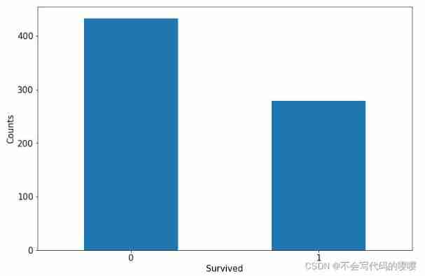
label Distribution situation
%matplotlib inline
%config InlineBackend.figure_format = 'png'
ax = dftrain_raw['Survived'].value_counts().plot(kind = 'bar',
     figsize = (12,8),fontsize=15,rot = 0)
ax.set_ylabel('Counts',fontsize = 15)
ax.set_xlabel('Survived',fontsize = 15)
plt.show()
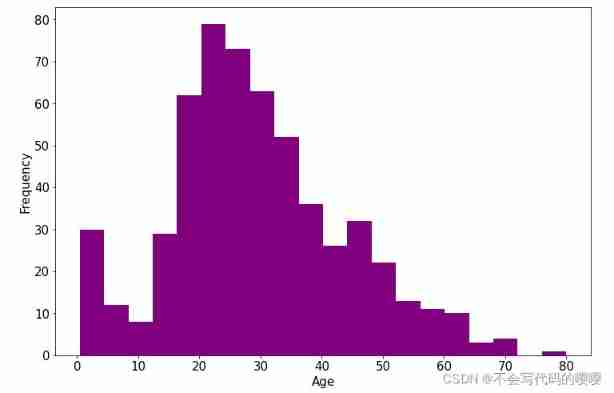
Age distribution
%matplotlib inline
%config InlineBackend.figure_format = 'png'
ax = dftrain_raw['Age'].plot(kind = 'hist',bins = 20,color= 'purple',
                    figsize = (12,8),fontsize=15)

ax.set_ylabel('Frequency',fontsize = 15)
ax.set_xlabel('Age',fontsize = 15)
plt.show()
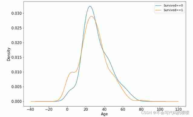
Age and label The relevance of
%matplotlib inline
%config InlineBackend.figure_format = 'png'
ax = dftrain_raw.query('Survived == 0')['Age'].plot(kind = 'density',
                      figsize = (12,8),fontsize=15)
dftrain_raw.query('Survived == 1')['Age'].plot(kind = 'density',
                      figsize = (12,8),fontsize=15)
ax.legend(['Survived==0','Survived==1'],fontsize = 12)
ax.set_ylabel('Density',fontsize = 15)
ax.set_xlabel('Age',fontsize = 15)
plt.show()
Next, data preprocessing
- For the above onehot code , It's used here pandas Of get_dummies Method
def preprocessing(dfdata):
dfresult= pd.DataFrame()
#Pclass
dfPclass = pd.get_dummies(dfdata['Pclass'])
dfPclass.columns = ['Pclass_' +str(x) for x in dfPclass.columns ]
dfresult = pd.concat([dfresult,dfPclass],axis = 1)
#Sex
dfSex = pd.get_dummies(dfdata['Sex'])
dfresult = pd.concat([dfresult,dfSex],axis = 1)
#Age
dfresult['Age'] = dfdata['Age'].fillna(0)
dfresult['Age_null'] = pd.isna(dfdata['Age']).astype('int32')
#SibSp,Parch,Fare
dfresult['SibSp'] = dfdata['SibSp']
dfresult['Parch'] = dfdata['Parch']
dfresult['Fare'] = dfdata['Fare']
#Carbin
dfresult['Cabin_null'] = pd.isna(dfdata['Cabin']).astype('int32')
#Embarked
dfEmbarked = pd.get_dummies(dfdata['Embarked'],dummy_na=True)
dfEmbarked.columns = ['Embarked_' + str(x) for x in dfEmbarked.columns]
dfresult = pd.concat([dfresult,dfEmbarked],axis = 1)
return(dfresult)
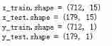
x_train = preprocessing(dftrain_raw).values
y_train = dftrain_raw[['Survived']].values
x_test = preprocessing(dftest_raw).values
y_test = dftest_raw[['Survived']].values
print("x_train.shape =", x_train.shape )
print("x_test.shape =", x_test.shape )
print("y_train.shape =", y_train.shape )
print("y_test.shape =", y_test.shape )
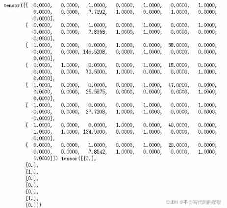
Further use DataLoader and TensorDataset Data can be encapsulated into a pipeline .
dl_train = DataLoader(TensorDataset(torch.tensor(x_train).float(),torch.tensor(y_train).float()),
                     shuffle = True, batch_size = 8)
dl_valid = DataLoader(TensorDataset(torch.tensor(x_test).float(),torch.tensor(y_test).float()),
                     shuffle = False, batch_size = 8)
#  Test data pipeline
for features,labels in dl_train:
    print(features,labels)
    break
2. Defining models
Pytorch There are usually three ways to build models :
- Use nn.Sequential Build models in a hierarchical order
- Inherit nn.Module Base classes build custom models
- Inherit nn.Module The base class builds the model and assists in encapsulating the model container .
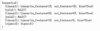
Here choose the easiest to use nn.Sequential, Hierarchical order model .
def create_net():
    net = nn.Sequential()
    net.add_module("linear1",nn.Linear(15,20))
    net.add_module("relu1",nn.ReLU())
    net.add_module("linear2",nn.Linear(20,15))
    net.add_module("relu2",nn.ReLU())
    net.add_module("linear3",nn.Linear(15,1))
    net.add_module("sigmoid",nn.Sigmoid())
    return net

net = create_net()
print(net)
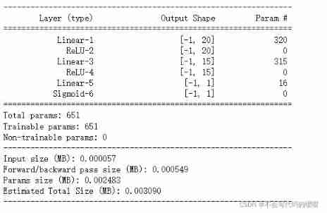
from torchkeras import summary
summary(net,input_shape=(15,))
3. Training models
Pytorch It usually requires the user to write a custom training cycle , The code style of the training cycle varies from person to person .
Yes 3 Class typical training cycle code style :
- Script form training cycle
- Function form training cycle
- Class form training cycle .
Here is a more general script form .
Define the loss function and optimizer 、 Metric function
from sklearn.metrics import accuracy_score

loss_func = nn.BCELoss()
optimizer = torch.optim.Adam(params=net.parameters(),lr = 0.01)
metric_func = lambda y_pred,y_true: accuracy_score(y_true.data.numpy(),y_pred.data.numpy()>0.5)
metric_name = "accuracy"
Start training model
epochs = 10
log_step_freq = 30
dfhistory = pd.DataFrame(columns = ["epoch","loss",metric_name,"val_loss","val_"+metric_name])
print("Start Training...")
nowtime = datetime.datetime.now().strftime('%Y-%m-%d %H:%M:%S')
print("=========="*8 + "%s"%nowtime)
for epoch in range(1,epochs+1):
# 1, Training cycle -------------------------------------------------
net.train()
loss_sum = 0.0
metric_sum = 0.0
step = 1
for step, (features,labels) in enumerate(dl_train, 1):
# Gradient clear
optimizer.zero_grad()
# Forward propagation for loss
predictions = net(features)
loss = loss_func(predictions,labels)
metric = metric_func(predictions,labels)
# Back propagation gradient
loss.backward()
optimizer.step()
# Print batch The level of log
loss_sum += loss.item()
metric_sum += metric.item()
if step%log_step_freq == 0:
print(("[step = %d] loss: %.3f, "+metric_name+": %.3f") %
(step, loss_sum/step, metric_sum/step))
# 2, Verification cycle -------------------------------------------------
net.eval()
val_loss_sum = 0.0
val_metric_sum = 0.0
val_step = 1
for val_step, (features,labels) in enumerate(dl_valid, 1):
# Turn off gradient computation
with torch.no_grad():
predictions = net(features)
val_loss = loss_func(predictions,labels)
val_metric = metric_func(predictions,labels)
val_loss_sum += val_loss.item()
val_metric_sum += val_metric.item()
# 3, Log -------------------------------------------------
info = (epoch, loss_sum/step, metric_sum/step,
val_loss_sum/val_step, val_metric_sum/val_step)
dfhistory.loc[epoch-1] = info
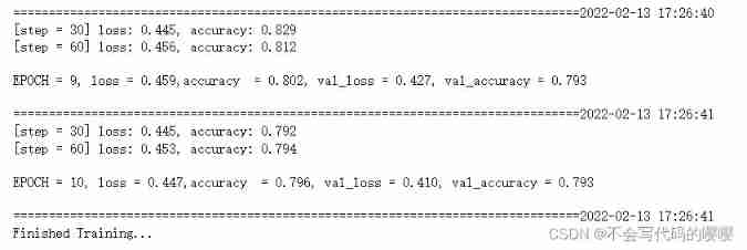
# Print epoch The level of log
print(("\nEPOCH = %d, loss = %.3f,"+ metric_name + \
" = %.3f, val_loss = %.3f, "+"val_"+ metric_name+" = %.3f")
%info)
nowtime = datetime.datetime.now().strftime('%Y-%m-%d %H:%M:%S')
print("\n"+"=========="*8 + "%s"%nowtime)
print('Finished Training...')
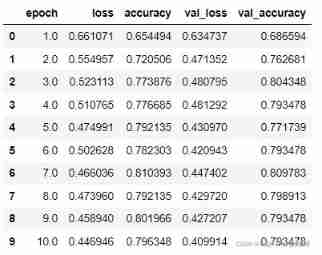
4. Model to evaluate
dfhistory
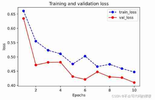
View loss curve
%matplotlib inline
%config InlineBackend.figure_format = 'svg'

import matplotlib.pyplot as plt

def plot_metric(dfhistory, metric):
    train_metrics = dfhistory[metric]
    val_metrics = dfhistory['val_'+metric]
    epochs = range(1, len(train_metrics) + 1)
    plt.plot(epochs, train_metrics, 'bo--')
    plt.plot(epochs, val_metrics, 'ro-')
    plt.title('Training and validation '+ metric)
    plt.xlabel("Epochs")
    plt.ylabel(metric)
    plt.legend(["train_"+metric, 'val_'+metric])
    plt.show()
plot_metric(dfhistory,"loss")
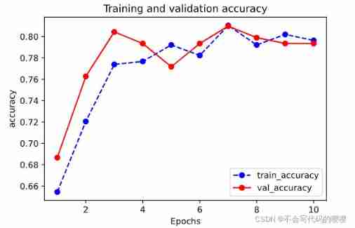
View accuracy curve
plot_metric(dfhistory,"accuracy")
5. Using the model
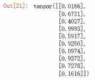
# Prediction probability
y_pred_probs = net(torch.tensor(x_test[0:10]).float()).data
y_pred_probs
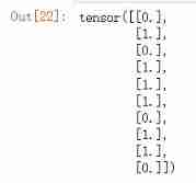
# Forecast category
y_pred = torch.where(y_pred_probs>0.5,
        torch.ones_like(y_pred_probs),torch.zeros_like(y_pred_probs))
y_pred
6. Model preservation
Pytorch There are two ways to save models , All by calling pickle The serialization method implements .
The first method only saves model parameters .
The second way to save the entire model .
The first one is recommended , The second method may cause various problems when switching devices and directories .
- Save model parameters ( recommend )
 #  Save model parameters

torch.save(net.state_dict(), "./data/net_parameter.pkl")
#  Creating networks
net_clone = create_net()
#  Load network parameters
net_clone.load_state_dict(torch.load("./data/net_parameter.pkl"))
#  Forward algorithm
net_clone.forward(torch.tensor(x_test[0:10]).float()).data
- Save the complete model ( Not recommended )
torch.save(net, './data/net_model.pkl')
net_loaded = torch.load('./data/net_model.pkl')
net_loaded(torch.tensor(x_test[0:10]).float()).data
Summary
A complete modeling process is given at the beginning, which is really a little confused , But after learning, I probably understand , The first day of study can be said to be understanding , Let us know pytorch A general process in structured data modeling , Generally speaking, it's the same as tensflow There are many similarities , Punch in the first day , come on. !
Source of learning
边栏推荐
- Summary of phased use of sonic one-stop open source distributed cluster cloud real machine test platform
- P3047 [usaco12feb]nearby cows g (tree DP)
- How to use information mechanism to realize process mutual exclusion, process synchronization and precursor relationship
- 数据治理:误区梳理篇
- All the ArrayList knowledge you want to know is here
- Migrate data from a tidb cluster to another tidb cluster
- Data governance: misunderstanding sorting
- Data governance: data quality
- Circular reference of ES6 module
- [Yugong series] February 2022 U3D full stack class 010 prefabricated parts
猜你喜欢
23. Update data
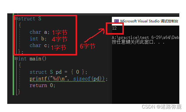
C language custom type: struct
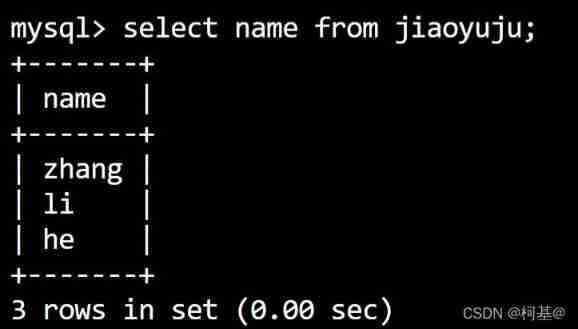
24. Query table data (basic)
![[research materials] 2022 China yuancosmos white paper - Download attached](/img/b4/422dff0510bbe67f3578202d6e80b7.jpg)
[research materials] 2022 China yuancosmos white paper - Download attached
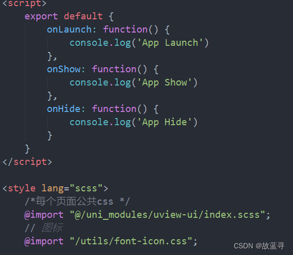
在 uniapp 中使用阿里图标
![[cloud native] teach you how to build ferry open source work order system](/img/fb/507f763791235bd00bc8201e5d7741.png)
[cloud native] teach you how to build ferry open source work order system
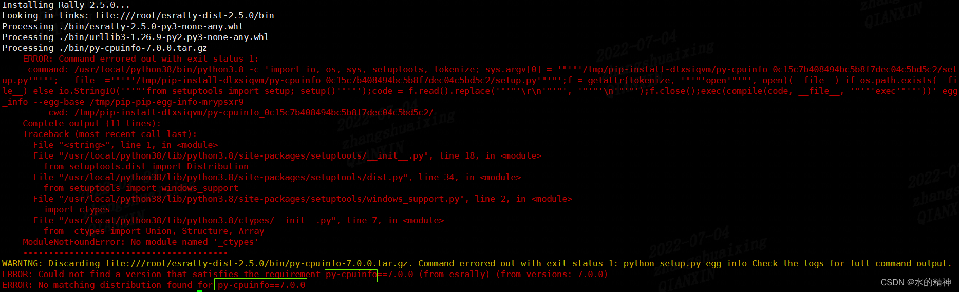
Esrally domestic installation and use pit avoidance Guide - the latest in the whole network
2.10transfrom attribute
Yyds dry goods inventory three JS source code interpretation eventdispatcher
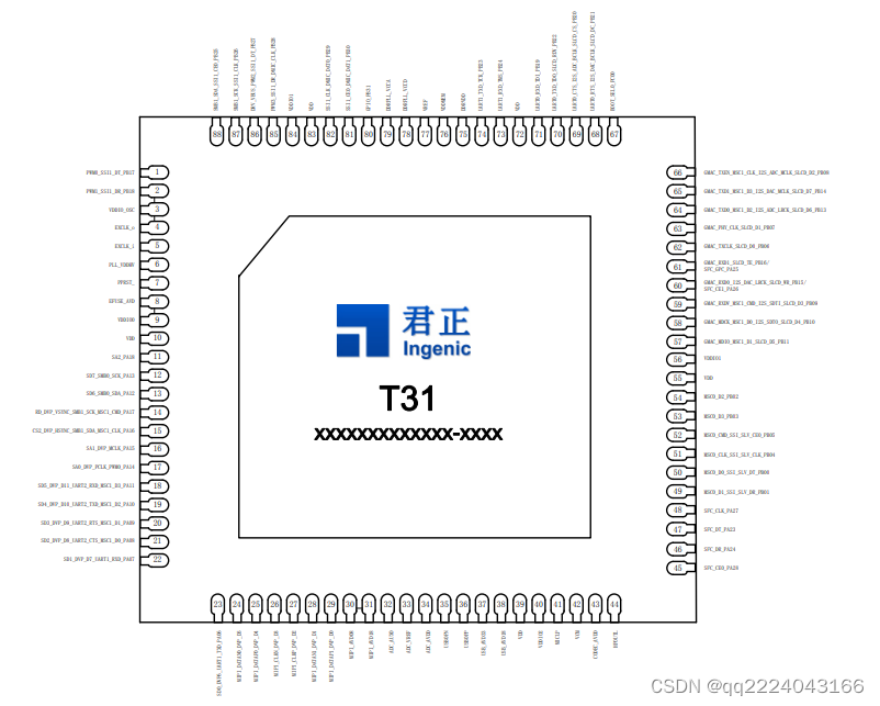
【T31ZL智能视频应用处理器资料】
随机推荐
化不掉的钟薛高,逃不出网红产品的生命周期
hcip--mpls
CAD ARX 获取当前的视口设置
Grayscale upgrade tidb operator
使用 TiDB Lightning 恢复 S3 兼容存储上的备份数据
Use dumping to back up tidb cluster data to S3 compatible storage
ESP series pin description diagram summary
C language - bit segment
[nonlinear control theory]9_ A series of lectures on nonlinear control theory
Upgrade tidb operator
Golang DNS 随便写写
Erc20 token agreement
Wincc7.5 download and installation tutorial (win10 system)
指针和数组笔试题解析
All the ArrayList knowledge you want to know is here
22. Empty the table
24. Query table data (basic)
Learn Arduino with examples
Summary of phased use of sonic one-stop open source distributed cluster cloud real machine test platform
【MySQL】数据库的存储过程与存储函数通关教程(完整版)