[local differential privacy and random response code implementation] differential privacy code implementation series (13)

Let me write it out front

When books come to school, they feel shallow , We must know that we must do it .

review

1、 Gradient descent is a method to reduce the loss by updating the model according to the gradient of loss . Gradient is like a multidimensional derivative ： For functions with multidimensional inputs （ Such as the loss function above ）, The gradient reflects the change speed of the output of the function relative to each dimension of the input . If the gradient is positive in a particular dimension , It means that if we increase the model weight of this dimension , Then the value of this function will increase ; We hope the loss will be reduced , So we should modify our model by moving in the opposite direction of the gradient , That is, do something opposite to the gradient . Because we move the model in the opposite direction of the gradient , So this is called gradient descent .

2、 Generally speaking , More training iterations can improve accuracy , But more iterations require more computing time . Most are used to make large-scale deep learning practical " skill " In fact, it is to speed up each iteration of gradient descent , In order to perform more iterations in the same time .

3、 Our goal is to make the final model not show any information about a single training example . The only part of the algorithm that uses training data is gradient calculation . One way to make the algorithm have differential privacy is to add noise to the gradient itself before updating the model at each iteration . This method is usually called noise gradient reduction , Because we add noise directly to the gradient .

4、 There are two main challenges . First , Gradient is the result of average query , It is the average of many gradients for each example . As we've seen before , It is best to split such queries into sum queries and count queries . It's not hard to do , We can calculate the sum of the gradients for each example , Not their average , And then divide by the noise count . secondly , We need to bind the sensitivity of each sample gradient . There are two basic ways ： We can analyze the gradient function itself （ As we did in the previous query ） To determine its worst-case global sensitivity , Or we can enforce sensitivity by tailoring the output of the gradient function （ As we did in samples and aggregations ）.

5、 Each iteration of the gradient clipping algorithm meets $(ϵ,\delta )$- Differential privacy , We perform an additional query to determine that $ϵ$- Differential privacy noise count . If we implement $k$ iteration , Then through sequential combination , Algorithm satisfaction $(kϵ+ϵ,k\delta )$- Differential privacy . We can also use advanced combinations to analyze the total privacy cost ; What's better is , We can convert the algorithm into Rényi Differential privacy or zero set differential privacy , And get strict restrictions on privacy costs .

6、 Our previous method is very general , Because it makes no assumptions about the behavior of gradients . However , Sometimes we do know something about the behavior of gradients . especially , A large class of useful gradient functions （ Including the gradient of logical loss we use here ） Lipschitz continuous , This means that they have bounded global sensitivity .

7、 Tailoring training examples rather than gradients has two advantages . First , Estimate the proportion of training data （ So as to choose a good cutting parameter ） It is usually easier to estimate the scale of the gradient to be calculated during training . secondly , It is more computationally efficient ： We can cut a training example , And reuse the tailored training data every time you train the model . Use gradient clipping , We need to trim each gradient during training . Besides , We are no longer forced to calculate the gradient of each example , So that we can cut them , contrary , We can calculate all gradients at once , This can be done very effectively （ This is a common skill in machine learning , But we won't discuss it here ）.

8、 Can reasonably be expected ,$ϵ$ The smaller the value of , The lower the accuracy of the model （ Because this is the trend of every differential privacy algorithm we have seen so far ）. This is the truth , But there is also a slightly more subtle trade-off , This is due to the composition we need to consider when performing multiple iterations of the algorithm ： More iterations mean greater privacy costs . In the standard gradient descent algorithm , More iterations , It usually produces better models . In our differential privacy version , More iterations may make the model worse , Because we have to use smaller for each iteration $ϵ$, Therefore, the scale of noise will rise . In differential privacy machine learning , It is important to strike a proper balance between the number of iterations used and the scale of noise added （ Sometimes it is very challenging ）.

Local differential privacy

up to now , The model mentioned above only considers the central model of differential privacy （ I prefer to call it central differential privacy ~）, Sensitive data is collected in a single data set .

In this setting , We assume that the analyst is malicious , But there is a trusted data manager who holds the data set and correctly implements the differential privacy mechanism specified by the analyst .

This setting is usually unrealistic . in many instances , Data managers and analysts are the same , In fact, there is no trusted third party to save data and execution mechanism .

in fact , The organizations that collect the most sensitive data are often the ones we don't trust , Of course, such an organization cannot act as a trusted data manager .

An alternative to the central model of differential privacy is the local model of differential privacy , Where the data becomes differential privacy before leaving the control of the data subject .

for example , You may send the data on the device to the data management organization , First add noise to the data . In the local model , Data managers don't need trust , Because the data they collect has met the requirements of differential privacy .

therefore , Compared with the central model , Local models have a huge advantage ： Data subjects in addition to themselves , No need to trust others .

This advantage makes it very popular in real-world deployment , Including the deployment of Google and apple .

Unfortunately , The local model also has an obvious disadvantage ： Under the central differential privacy , For the same privacy cost as the same query , The accuracy of query results in local models is usually several orders of magnitude lower .

This huge loss of accuracy means that only a few query types are suitable for local differential privacy , Even for these query types , It also requires a large number of participants .

In this blog , We will see two mechanisms for local differential privacy . The first is called （randomized response） random response , The second is called （unary encoding） Unary code .

random response

1965 year S. L. Warner The random response mentioned in this paper is a local differential privacy mechanism .

at that time , This technology aims to improve the bias in the survey responses to sensitive issues , And it was not initially proposed as a mechanism for differential privacy . After developing differential privacy , Statisticians realize that this existing technology has met the definition .

Dwork and Roth A variant of random response is proposed , The data subject answers " yes " or " no " problem , As shown below ：

1、 Flip a coin ~

2、 If the coin is on the obverse （ A head ）, Please answer the question truthfully .

3、 If the coin is on the reverse , Please toss another coin .

4、 If the second coin is positive , answer " yes ", Otherwise answer " no ".

The randomization in this algorithm comes from two coin flips . Like all other differential privacy algorithms , This randomization creates uncertainty about the true answer , The real answer is the source of privacy .

The fact proved that , This random response algorithm satisfies $ϵ$- Differential privacy $ϵ=\log (3)=1.09$.

Let's work for a simple " yes " or " no " Problem implementation algorithm ：" Your occupation is ’ sales ’ Do you ？ We can do it in Python Use in np.random.randint(0, 2), The result is 0 or 1.

%matplotlib inline
import matplotlib.pyplot as plt
plt.style.use('seaborn-whitegrid')
import pandas as pd
import numpy as np

adult = pd.read_csv("adult_with_pii.csv")
def laplace_mech(v, sensitivity, epsilon):
    return v + np.random.laplace(loc=0, scale=sensitivity / epsilon)
def pct_error(orig, priv):
    return np.abs(orig - priv)/orig * 100.0
def rand_resp_sales(response):
    truthful_response = response == 'Sales'
    
    #  First coin toss 
    if np.random.randint(0, 2) == 0:
        #  If you throw the front and answer the correct answer 
        return truthful_response
    else:
        #  Second coin toss 
        return np.random.randint(0, 2) == 0

Let's make 200 People who work in sales use random responses to answer , And look at the results .

pd.Series([rand_resp_sales('Sales') for i in range(200)]).value_counts()

What we see is that , We get " yes " and " no ", but " yes " Than " no " It is more important .

This output shows two features of the differential privacy algorithm we have seen ： It includes uncertainty , This protects privacy , But it also shows enough signals , So that we can infer something about people .

Let's try the same thing on some actual data . We will get all the occupations in the U.S. census data set that we have been using , And for every profession " Your occupation is ’ sales ’ Do you ？" Code the answer to the question .

In the actual deployed system , We will not collect this data set at all . contrary , Each respondent will run locally rand_resp_sales, And submit its random response to the data manager . For experiment , We will run on existing datasets rand_resp_sales.

responses = [rand_resp_sales(r) for r in adult['Occupation']]
pd.Series(responses).value_counts()

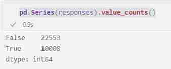
This time, , What we got " no " Than " yes " A lot more . After some thinking , It makes sense , Because most participants in the data set are not in sales .

The key question now is ： How can we estimate the exact number of salespeople in the data set based on these reactions ？ Obviously, what we have so far " yes " The number of is not a good estimate for the number of salespeople ：

len(adult[adult['Occupation'] == 'Sales'])

That's not surprising , Because many " yes " Random coin flip from Algorithm .

In order to estimate the real number of salespeople , We need to analyze the randomness of random response algorithm , And estimate how many " yes " The response comes from the actual salesperson , And how many are fake coins tossed randomly “ yes ”. We know ：

1、 The probability of random response of each responder is $\frac{1}{2}$

2、 Every random response is " yes " Is the probability that $\frac{1}{2}$

therefore , The respondent answered randomly " yes " Probability （ Not because they are salesmen ） yes $\frac{1}{2}\cdot \frac{1}{2}=\frac{1}{4}$. This means that we can expect a quarter of our total responses to be false " yes ".

responses = [rand_resp_sales(r) for r in adult['Occupation']]

# we expect 1/4 of the responses to be "yes" based entirely on the coin flip
# these are "fake" yesses
fake_yesses = len(responses)/4

# the total number of yesses recorded
num_yesses = np.sum([1 if r else 0 for r in responses])

# the number of "real" yesses is the total number of yesses minus the fake yesses
true_yesses = num_yesses - fake_yesses

Another factor we need to consider is , Half of the respondents answered randomly , But some random interviewees may actually be salespeople . How many of them are salesmen ？ We have no data on this , Because they answered at random ！

however , Because we randomly divided the respondents into " The truth " and " Random " Group （ By tossing a coin for the first time ）, We can hope that the number of salespeople in the two groups is roughly the same . therefore , If we can estimate " The truth " Number of salespeople in the Group , You can double this number , To get the total number of salespeople .

rr_result = true_yesses*2
rr_result

How close is this to the real number of salespeople ？ Let's compare ！

true_result = np.sum(adult['Occupation'] == 'Sales')
true_result

pct_error(true_result, rr_result)

Using this method , And a considerable number （ for example , In this case more than 3000）, We usually get " acceptable " The error rate of is lower than 5%. If your goal is to identify the most popular occupation , Then this method may be effective . however , When the count is small , The error will soon increase .

Besides , The random response is several orders of magnitude worse than the Laplace mechanism in the central model . Let's compare the two in this example ：

pct_error(true_result, laplace_mech(true_result, 1, 1))

ad locum , The error we get is about 0.01%, Even if we are interested in the central model $ϵ$ The value is slightly lower than that we use for random response $ϵ$ value .

Local models have better algorithms , However, the inherent limitation of adding noise before submitting data means that the accuracy of the local model algorithm is always worse than that of the best central model algorithm .

Unary code

Random responses allow us to propose that privacy with local differences is / No problem . What if we want to build histograms ？

Many different algorithms have been proposed , Used to solve this problem in the local model of differential privacy .

Wang Et al. 2017 A paper in summarizes some of the best methods .

ad locum , I will study the simplest of them , It is called unary coding . This way is Google Of RAPPOR Foundation of the system （ With some modifications , Make it better applicable to large domains and multiple responses over time ）.

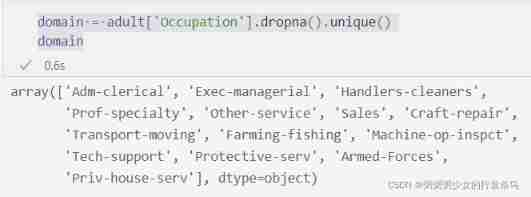
The first step is to define the domain of the response , That is, we are concerned about the labels of histogram bars .

For our example , We want to know how many participants are associated with each profession , So our domain is a career set .

domain = adult['Occupation'].dropna().unique()
domain

We will define three functions , Together, they implement the unary coding mechanism ：

1、encode, Encode the response

2、perturb, This will disturb the response of the code

3、aggregate, Reconstruct the final result from the disturbance response

The name of this technology comes from the coding method used ： For one $k$ Size fields , Each response is encoded as $k$ Bit length vector , In addition to the position corresponding to the profession of the respondent , All positions are 0. In machine learning , This representation is called "one-hot encoding".

for example ,"Sales" Is the second of the domain 6 Elements , therefore "Sales" Occupation use 6 Elements are 1 The vector of .

def encode(response):
    return [1 if d == response else 0 for d in domain]

encode('Sales')

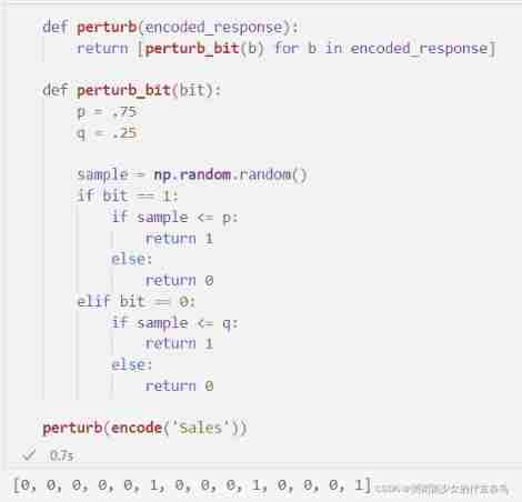
The next step is to perturb , It flips the bits in the response vector to ensure differential privacy . The probability of bits being flipped is based on two parameters $p$ and $q$, Together, they determine privacy parameters $ϵ$（ Based on the formula we will see later ）.
$$\mathsf{P}\mathsf{r}[B^{\prime }[i]=1]=\{\begin{array}{l}p\text{if}B[i]=1\\ q\text{if}B[i]=0\end{array}$$

def perturb(encoded_response):
    return [perturb_bit(b) for b in encoded_response]

def perturb_bit(bit):
    p = .75
    q = .25

    sample = np.random.random()
    if bit == 1:
        if sample <= p:
            return 1
        else:
            return 0
    elif bit == 0:
        if sample <= q:
            return 1
        else: 
            return 0

perturb(encode('Sales'))

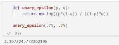
according to $p$ and $q$ Value , We can calculate the value of privacy parameter $ϵ$. about $p=.75$ and $q=.25$, We will see slightly larger 2 One of the $ϵ$.
$$ϵ=\log \left(\frac{p(1-q)}{(1-p)q}\right)$$

def unary_epsilon(p, q):
    return np.log((p*(1-q)) / ((1-p)*q))

unary_epsilon(.75, .25)

The last part is aggregation . If we don't make any disturbance , Then we can simply get the set of response vectors and add them one by one , To get the count of each element in the field ：

counts = np.sum([encode(r) for r in adult['Occupation']], axis=0)
list(zip(domain, counts))

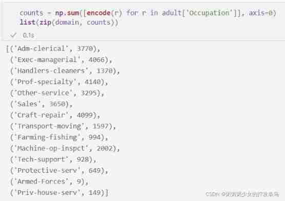
But as we can see in the random response , Caused by inversion " false " The response makes the result difficult to interpret . If we perform the same process for the disturbance response , Then the count is all wrong ：

counts = np.sum([perturb(encode(r)) for r in adult['Occupation']], axis=0)
list(zip(domain, counts))

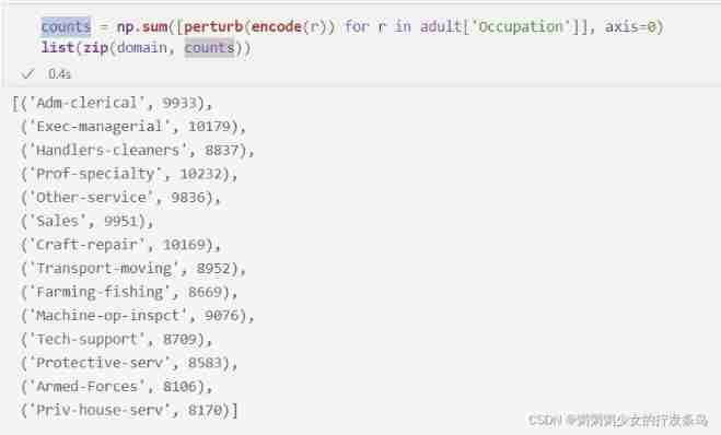
The aggregation step of the unary coding algorithm considers " false " Number of responses , This is a $p$ and $q$ Function of , And the number of responses $n$：
$$A[i]=\frac{{\sum }_j{B}_j^{\prime }[i]-nq}{p-q}$$

def aggregate(responses):
    p = .75
    q = .25
    
    sums = np.sum(responses, axis=0)
    n = len(responses)
    
    return [(v - n*q) / (p-q) for v in sums] 
    
responses = [perturb(encode(r)) for r in adult['Occupation']]
counts = aggregate(responses)
list(zip(domain, counts))

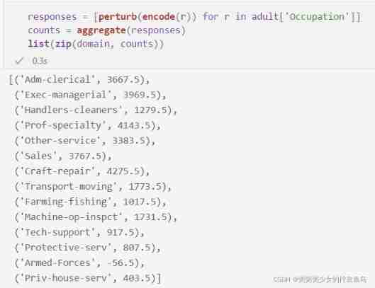
As we can see in the random response , These results are accurate enough , You can get the domain element （ At least the most popular domain element ） Rough sort of , But it is several orders of magnitude lower than the accuracy obtained by using Laplace mechanism in the differential privacy center model .

Other methods for performing histogram queries in local models have been proposed , Including some methods detailed in the previous paper . These can improve the accuracy to a certain extent , However, in the local model, the basic limitation of differential privacy of each sample must be ensured, which means , Even the most complex technologies cannot match the accuracy of the mechanisms we see in the central model .

summary

1、 The local model also has an obvious disadvantage ： Under the central differential privacy , For the same privacy cost as the same query , The accuracy of query results in local models is usually several orders of magnitude lower . This huge loss of accuracy means that only a few query types are suitable for local differential privacy , Even for these query types , It also requires a large number of participants .

2、 When the answer itself is small , The error of the local model will increase . In error , The random response is several orders of magnitude worse than the Laplace mechanism in the central model . Even if the local model has better algorithms , However, the inherent limitation of adding noise before submitting data means that the accuracy of the local model algorithm is always worse than that of the best central model algorithm .

3、 Other methods for performing histogram queries in local models have been proposed , Including some methods detailed in the previous paper . These can improve the accuracy to a certain extent , However, in the local model, the basic limitation of differential privacy of each sample must be ensured, which means , Even the most complex technologies cannot match the accuracy of the mechanisms we see in the central model .