当前位置:网站首页>Quick introduction to automatic control principle + understanding
Quick introduction to automatic control principle + understanding
2022-07-04 14:49:00 【Pony Baby】
Know the whole picture in the simplest words .
PS: The default is linear system , That is, the input and output are linear ( By default, you know what is linear ).
Preliminary understanding of control
Suppose you are pushing a box , Your pushing force is f f f, Case displacement is x x x, Quality is 1 1 1, No friction , Then according to simple physics :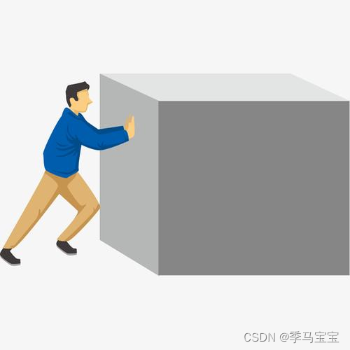
f = m a = x ¨ f=ma=\ddot{x} f=ma=x¨
One thing that needs special attention , Whether it's f still x It's all about time t Function of , This formula actually looks like this , This is it. Model of the system :
f ( t ) = m a = x ¨ ( t ) f(t)=ma=\ddot{x}(t) f(t)=ma=x¨(t)
hypothesis f ( t ) = 1 f(t)=1 f(t)=1, The solution is x ( t ) = 1 2 t 2 x(t)=\frac{1}{2}t^2 x(t)=21t2, Get a very important output function about time .
Let's think about a problem , because F It won't be the same every time , The force we push can be any function of time , Should we bring it in every time F To solve a complex differential equation , Is there a better way ? The answer is Laplace transform .
Laplace transform a lot , Remember a few key , The rest is to check the table . But the differential property of Laplace transform must be known A top priority . Just remember the following two , The same is true for higher-order forms , However, the topic generally does not have . If it is really high-level, it must be solved by software .
L [ d f ( t ) d t ] = s F ( s ) − f ( 0 ) L\left[\frac{d f(t)}{d t}\right]=s F(s)-f(0) L[dtdf(t)]=sF(s)−f(0),
L [ d 2 f ( t ) d t ] = s 2 F ( s ) − s f ( 0 ) − f ′ ( 0 ) L\left[\frac{d^{2} f(t)}{d t}\right]=s^{2} F(s)-s f(0)-f^{\prime}(0) L[dtd2f(t)]=s2F(s)−sf(0)−f′(0)
Let's solve it with Laplace transform ( Unified lowercase represents time domain , Capital stands for s Domain ), We assume that the initial values are 0:
F ( t ) = s 2 X ( s ) − s x ( 0 ) − x ˙ ( 0 ) = s 2 X ( s ) F(t)=s^2X(s)-sx(0)-\dot{x}(0)=s^2X(s) F(t)=s2X(s)−sx(0)−x˙(0)=s2X(s)
G ( s ) = X ( s ) F ( s ) = 1 s 2 G(s)=\frac{X(s)}{F(s)}=\frac{1}{s^2} G(s)=F(s)X(s)=s21
Now you know s The ratio of output to input in the field , When your output f ( t ) f(t) f(t) After changing , You just need to find the Laplace transform F ( s ) F(s) F(s) Bring it in to find X ( s ) X(s) X(s), Then pull the inverse transformation to get the result . Whatever you are f ( t ) f(t) f(t) How to change , Not right G ( s ) G(s) G(s) An impact , This is in this system An unchanging formula , That is, it represents the internal nature of the system .
Let's try f ( t ) = 1 f(t)=1 f(t)=1, be F ( s ) = 1 s F(s)=\frac{1}{s} F(s)=s1, be X ( s ) = G ( s ) F ( s ) = 1 s 3 X(s)=G(s)F(s)=\frac{1}{s^3} X(s)=G(s)F(s)=s31, Find the pull inverse transformation x ( t ) = 1 2 t 2 x(t)=\frac{1}{2}t^2 x(t)=21t2
For the control system , Our task is to stabilize the output at a certain value , For example, we push an object in the hope that it will just stop somewhere , But now f ( t ) f(t) f(t) Obviously divergent , That is to say, the system is Unstable , We will talk more about stability later .
Control what needs to be done :
Of course you want to push the box gently, and finally your strength will return 0, But this system has no friction , therefore x Never stable , This system is simply not stable . So you need Make changes to the system , For example, add friction . And you should also change the way you push boxes , You may need to push quickly, but the box will be unstable , Push slowly for a long time . And these are the things that control has to do .
Amplitude frequency response and phase frequency response
Think about how our robots are controlled ? Circuit, of course . Generally speaking, the circuit must be AC , That is, the combination of sinusoidal signals with different frequencies ( Of course, any wave can become a combination of sinusoidal signals through Fourier transform , so much the better ). Experiments and theories tell us that for linear systems , Input sine wave , The output is also a sine wave of the same frequency , What has changed is only Amplitude and phase ( It's easy to understand the second superposition of linear systems ). that , If we know the response of the system to different frequency signals, we can easily analyze the relationship between input and output ?
Let's change to a more complex system :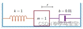
System equations :
m ⋅ d 2 r d t 2 + b ⋅ d r d t + k ⋅ r = k F ( t ) m \cdot \frac{d^{2} r}{d t^{2}}+b \cdot \frac{d r}{d t}+k \cdot r=k F(t) m⋅dt2d2r+b⋅dtdr+k⋅r=kF(t)
Transfer function :
Y ( s ) = R ( s ) F ( s ) = k m s 2 + b s + k = ω n 2 s 2 + 2 ξ ω n s + ω n 2 Y(s)=\frac{R(s)}{F(s)}=\frac{k}{m s^{2}+b s+k}=\frac{\omega_{n}^{2}}{s^{2}+2 \xi_{\omega_{n}} s+\omega_{n}^{2}} Y(s)=F(s)R(s)=ms2+bs+kk=s2+2ξωns+ωn2ωn2
among ω n = k m , ξ = b 2 k m \omega_{n}=\sqrt{\frac{k}{m}},\xi=\frac{b}{2\sqrt{km}} ωn=mk,ξ=2kmb
Into the s = j ω s=j\omega s=jω, be :( It's very important here , The Laplace transform after the change is actually The Fourier transform , That is, it is expanded according to the frequency )
∣ Y ( j ω ) ∣ = 1 ( 1 − ( ω ω n ) 2 ) 2 + 4 ξ 2 ( ω ω n ) 2 , ∠ Y ( j ω ) = − artan 2 ξ ω ω n 1 − ( ω ω n ) 2 |Y(j \omega)|=\frac{1}{\sqrt{\left(1-\left(\frac{\omega}{\omega_{n}}\right)^{2}\right)^{2}+4 \xi^{2}\left(\frac{\omega}{\omega_{n}}\right)^{2}}},\angle Y(j \omega)=-\operatorname{artan} \frac{2 \xi \frac{\omega}{\omega_{n}}}{1-\left(\frac{\omega}{\omega_{n}}\right)^{2}} ∣Y(jω)∣=(1−(ωnω)2)2+4ξ2(ωnω)21,∠Y(jω)=−artan1−(ωnω)22ξωnω
One of the above two formulas is amplitude , One is phase , For an input frequency , These are two fixed values . Let's draw these two functions .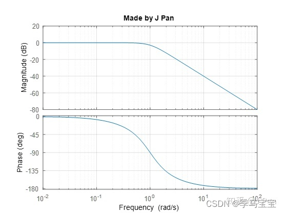
It's on it Amplitude response Set the output ratio input to K, The amplitude is taken 20logK, Because the range of values is very large , This is Porto . When input equals output , Namely 0.
Here is Frequency response , Because it's a causal signal , Always phase lag ( The phase lag in frequency domain is represented by the time delay in time domain , Your state starts with 0 You can't turn into 1 Well , There must be a time difference ).
We can find that this is a low-pass system , The input signal with low frequency can pass , Those with high frequency basically have no attenuation .
Suppose the input is a step signal :
The output looks like this , The low-frequency signal is retained , You can change the system delay time by modifying the system parameters , But overshoot ( Spit out part ) Will increase , How to balance is also what you need to consider when designing the control system :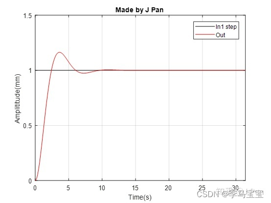
system stability
Pole-Zero :
G ( s ) = ( s − b 1 ) ( s − b 2 ) 2 ( s − a 1 ) ( s − a 2 ) 2 G(s)=\frac{(s-b_1)(s-b_2)^2}{(s-a_1)(s-a_2)^2} G(s)=(s−a1)(s−a2)2(s−b1)(s−b2)2
s = b 1 s=b_1 s=b1 Is the first order zero , s = b 2 s=b_2 s=b2 Is the second order zero , s = a 1 s=a_1 s=a1 Is the pole of the first order , s = a 2 s=a_2 s=a2 Is the second-order pole
If there is a i = b j a_i=b_j ai=bj, Then there is zero pole cancellation
Generally speaking , If the poles of the transfer function are all in the left half plane, it is stable , One is unstable in the right half plane . If there are poles at the origin, there will be steady-state components ( unstable ), There will be a sinusoidal signal on the vertical axis outside the origin ( Critical stability ). Well understood. , The following is the translation property of Laplace transform :
L [ f ( t ) e − a t ] = F ( s + a ) L\left[f(t) e^{-a t}\right]=F(s+a) L[f(t)e−at]=F(s+a)
once a<0, The pole of the right half will appear , There will also be instability e ∣ a ∣ t e^{|a|t} e∣a∣t component .
PS: If you study the principle of automatic control , You will learn many ways to judge stability , Because solving equations of very high degree manually ( But now we all use computers , So it's useless to actually use ). I don't want to spend a lot here , There are many contents in this part, which is of course very important for the exam , But don't go into detail , Just have an understanding first .
System stability and zero pole position :
The poles of the transfer function represent the mode of the system , in other words , When the frequency of the excitation is close to or the same as the frequency represented by the pole , The system will resonate , The response of the system reaches the maximum .
What does zero mean ?—— Contrary to the pole , Represents the mode that the system can shield , That is, the anti resonance point , let me put it another way , When the frequency of excitation is the same as that represented by zero , The system will have no response or very little response .
Taken together :** The transient response of the system depends on the mode represented by the pole ; The steady-state response depends on the distance between the excitation frequency and the zero and pole , The closer to the pole , The larger the steady-state response , The closer to zero , The smaller the steady-state response .** This obviously contradicts the idea that the closer we are to the pole, the more unstable we are ( Opposition ), So we should also make a balance .
So we assign the position of zero and pole , Satisfactory frequency response characteristics can be obtained . For example, we want to amplify a certain frequency ( Bandpass ) Put a pole at that frequency , We want a certain frequency to be suppressed ( Notch filter ) You can put a zero there , See the details later , Need to use feedback .
in addition , There are two points about simplification .
One is to delete too small zeros and poles , It's easy to think of , For example, your output function about time is x ( t ) = e − x + e − 10 x + e − 100 x x(t)=e^{-x}+e^{-10x}+e^{-100x} x(t)=e−x+e−10x+e−100x, Obviously your x It has the biggest relationship with the first item , The latter two items can be basically ignored . Generally speaking, small ones can be ignored if there is an order of magnitude difference .
Second, when the zero pole is close enough , It can be cancelled .
In addition, I will not go into detail about the knowledge of minimum phase system , You can see Minimum phase system understanding
feedback
More content , I'll add later , You can look at Refer to Zhihu JPAN
Here I add a little understanding of the examples in the article :
Suppose the transfer function of a system is : G ( s ) = 1 s + 1 G(s)=\frac{1}{s+1} G(s)=s+11
The step response of this system is :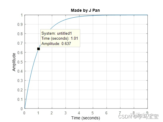
Response to stable value 63.2% The time required is about 1s, Very slowly , The reason is that the cut-off frequency is too low , Its Byrd picture is
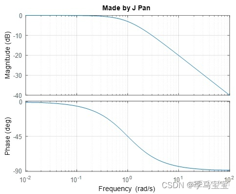
To solve this problem , We use the following results , This is a proportional control . If K It's big , It's equivalent to slamming on the accelerator , It will definitely reach the value we want very soon . But without control , In the end, we will exceed the expected speed , Something is needed to suppress , Negative feedback plays this role , If the output exceeds the input value , Then the excess part will become a reaction force and make your accelerator unable to step down .![so , When the input is greater than [ The formula ] when , The amplitude response of the system decays sharply , Let's suppose the input is [ The formula ] , The amplitude is attenuated to [ The formula ] , That is, the input 10%, Output is very small ! If we want to maintain the input at [ The formula ] , The output does not decay much , What shall I do? ?—— Negative feedback system !](/img/d9/67da331478dd0139cd0adfc7c50ab6.png)
When kp take 100 When , The cut-off frequency has increased significantly , Follow the characteristics to get better .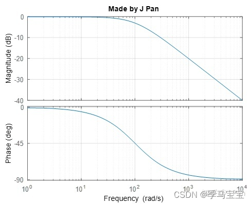
We said earlier , As long as the cut-off frequency is high enough , The output can follow the input very well , This statement is not very rigorous , Because the article said at the beginning , When each frequency component passes through the system , It's not just the amplitude that has attenuation , The phase is also delayed , If the phase delay is too much , After the signal is superimposed again, it may be quite different from the input . Therefore, the rigorous statement is : When the phase delay is within a certain range , The higher the cut-off frequency , The closer the output is to the input . How to quantify this matter ?—— Phase margin .
Mentioned earlier , Join in PI Behind the controller , The closed-loop transfer function of the system becomes very complex , Existing poles , There is zero again , It's not easy to analyze , therefore , Predecessors in the field of automatic control have come up with an idea , That is to design the cut-off frequency and phase margin of the open-loop front channel first , Then analyze the response of the closed-loop system .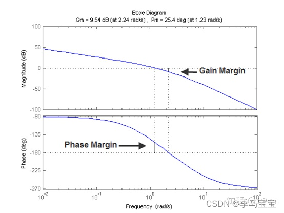
When the corrected system ( Controller and G(s) Open loop forward channel ) When the amplitude response of begins to decay ( The output amplitude is smaller than the input , That is to say 0dB), The phase delay of the signal is related to -180° The distance is the phase margin . so , The larger the phase margin, the better , Theoretically, if the phase margin reaches 180°, Then there is no phase delay , Of course, in fact, it can't be achieved , Generally speaking, the phase margin is 40° above , Of course, it will be different according to different applications . To sum up :
The amplitude response of the system can be constrained by the cut-off frequency , Phase response should be constrained by phase margin .
边栏推荐
- LVGL 8.2 LED
- First experience of ViewModel
- PLC Analog input analog conversion FC s_ ITR (CoDeSys platform)
- Solutions to the problems of miui12.5 red rice k20pro using Au or povo2
- 自动控制原理快速入门+理解
- C language book rental management system
- PyTorch的自动求导机制详细解析,PyTorch的核心魔法
- LVGL 8.2 Draw label with gradient color
- Sqlserver functions, creation and use of stored procedures
- Node mongodb installation
猜你喜欢
现代控制理论入门+理解
如何配和弦

如何配和弦

How to match chords
信号处理之一阶RC低通滤波器宏指令实现(繁易触摸屏)
![Leetcode 1200 minimum absolute difference [sort] the way of leetcode in heroding](/img/4a/6763e3fbdeaf9de673fbe8eaf96858.png)
Leetcode 1200 minimum absolute difference [sort] the way of leetcode in heroding
![leetcode:6110. The number of incremental paths in the grid graph [DFS + cache]](/img/48/56ed03b21709a97fd55c8cccf98092.png)
leetcode:6110. The number of incremental paths in the grid graph [DFS + cache]
Digi restarts XBee Pro S2C production. Some differences need to be noted

WT588F02B-8S(C006_03)单芯片语音ic方案为智能门铃设计降本增效赋能
Practical puzzle solving | how to extract irregular ROI regions in opencv
随机推荐
Docker compose public network deployment redis sentinel mode
Detailed analysis of pytorch's automatic derivation mechanism, pytorch's core magic
Digi XBee 3 rf: 4 protocols, 3 packages, 10 major functions
scratch古堡历险记 电子学会图形化编程scratch等级考试三级真题和答案解析2022年6月
Digi restarts XBee Pro S2C production. Some differences need to be noted
Nowcoder reverse linked list
Kubernets Pod 存在 Finalizers 一直处于 Terminating 状态
SAIC Maxus officially released its new brand "mifa", and its flagship product mifa 9 was officially unveiled!
LVGL 8.2 keyboard
WT588F02B-8S(C006_03)单芯片语音ic方案为智能门铃设计降本增效赋能
10. (map data) offline terrain data processing (for cesium)
Redis daily notes
Is it safe to open an account online for stock speculation? Will you be cheated.
《opencv学习笔记》-- 线性滤波:方框滤波、均值滤波、高斯滤波
LVGL 8.2 List
Graduation season - personal summary
es6模块化
阿里被裁员工,找工作第N天,猎头又传来噩耗...
Leecode learning notes - Joseph problem
[cloud native] how can I compete with this database?