当前位置:网站首页>R note prophet
R note prophet
2022-07-06 04:07:00 【UQI-LIUWJ】
0 Theoretical part
Paper notes :Forecasting at Scale(Prophet)_UQI-LIUWJ The blog of -CSDN Blog
Prophet It is a program based on additive model to predict time series data , Among them, nonlinear trend 、 Seasonal and holiday effects match .
It is most suitable for time series with strong seasonality and several seasonal historical data .
Prophet Robust to missing data and trend changes , And you can usually handle outliers very well .
1 The basic flow
stay R in , We use normal model fitting API. We provide a method to execute the model object to be merged and returned Prophet function . then , You can call on this model object predict and plot.
library(prophet)
1.1 Read in the data
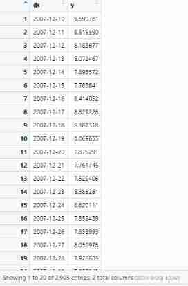
First , We read in the data and create the result variable . And Python Medium dataframe equally , This is an inclusion of ds and y Column data box , Include date and value respectively .
ds The column should be YYYY-MM-DD, For the moment, it should be YYYY-MM-DD HH:MM:SS.
df<-read.csv('C:/Users/16000/example_wp_log_peyton_manning.csv')
1.2 call prophet function
call prophet Function to fit the model ( Time series decomposition of the previous part )
m<-prophet(df)
1.3 Generate future dataframe
The prediction is dataframe On , among ds The column contains the date to forecast .
make_future_dataframe Function USES Model objects and Length of prediction interval Make predictions and generate corresponding dataframe.
future <- make_future_dataframe(m, periods = 365)By default , It will also include historical dates , Therefore, we can evaluate the fitting within the sample .
Compared with df, More 365 Data , That is, the prediction interval


1.4 Get forecast results
And R Most of the prediction tasks in are the same , We use universal predict Function to get our prediction .
forecast <- predict(m, future)The prediction result is dataframe, Which contains the predicted columns yhat. It has additional columns for uncertainty intervals and seasonal components .
tail(forecast)

             ds    trend additive_terms
3265 2017-01-14 7.188345      0.6353367
3266 2017-01-15 7.187317      1.0181583
3267 2017-01-16 7.186289      1.3441746
3268 2017-01-17 7.185261      1.1326084
3269 2017-01-18 7.184232      0.9662578
3270 2017-01-19 7.183204      0.9791888
     additive_terms_lower additive_terms_upper
3265            0.6353367            0.6353367
3266            1.0181583            1.0181583
3267            1.3441746            1.3441746
3268            1.1326084            1.1326084
3269            0.9662578            0.9662578
3270            0.9791888            0.9791888
          weekly weekly_lower weekly_upper    yearly
3265 -0.31171456  -0.31171456  -0.31171456 0.9470512
3266  0.04829728   0.04829728   0.04829728 0.9698610
3267  0.35228502   0.35228502   0.35228502 0.9918896
3268  0.11963367   0.11963367   0.11963367 1.0129747
3269 -0.06665548  -0.06665548  -0.06665548 1.0329133
3270 -0.07227149  -0.07227149  -0.07227149 1.0514603
     yearly_lower yearly_upper multiplicative_terms
3265    0.9470512    0.9470512                    0
3266    0.9698610    0.9698610                    0
3267    0.9918896    0.9918896                    0
3268    1.0129747    1.0129747                    0
3269    1.0329133    1.0329133                    0
3270    1.0514603    1.0514603                    0
     multiplicative_terms_lower
3265                          0
3266                          0
3267                          0
3268                          0
3269                          0
3270                          0
     multiplicative_terms_upper yhat_lower yhat_upper
3265                          0   7.054971   8.545286
3266                          0   7.443115   8.954531
3267                          0   7.791419   9.265397
3268                          0   7.664162   9.071099
3269                          0   7.391583   8.871629
3270                          0   7.428541   8.869961
     trend_lower trend_upper     yhat
3265    6.826222    7.538852 7.823682
3266    6.823645    7.538624 8.205475
3267    6.821068    7.538397 8.530463
3268    6.818564    7.538169 8.317869
3269    6.816108    7.537942 8.150490
3270    6.813651    7.537714 8.162393
Select a specific column , Sure
 tail(forecast[c('ds', 'yhat', 'yhat_lower', 'yhat_upper')])
             ds     yhat yhat_lower yhat_upper
3265 2017-01-14 7.823682   7.054971   8.545286
3266 2017-01-15 8.205475   7.443115   8.954531
3267 2017-01-16 8.530463   7.791419   9.265397
3268 2017-01-17 8.317869   7.664162   9.071099
3269 2017-01-18 8.150490   7.391583   8.871629
3270 2017-01-19 8.162393   7.428541   8.869961
1.5 The plot
1.5.1 plot
have access to plot function , Draw predictions by passing in models and prediction data frames .
plot(m, forecast)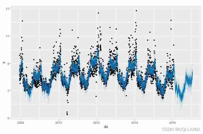
1.5.2 prophet_plot_components function
prophet_plot_components(m,forecast) 
2 The trend is a saturated growth model
The general framework and are the same , There are several small differences
Loading packages is the same as reading data
library(prophet)

df<-read.csv('C:/Users/16000/example_wp_log_peyton_manning.csv')
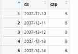
We need Add a column to the dataset : Carrying capacity C
Paper notes :Forecasting at Scale(Prophet)_UQI-LIUWJ The blog of -CSDN Blog
df['cap']=8
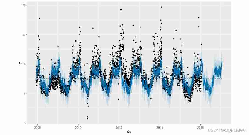
call prophet When , You need to declare a saturation growth model
m<-prophet(df,growth='logistic')
Generate future_dataframe When , It is also necessary to add the column of bearing capacity
future<-make_future_dataframe(m,period=365)
future['cap']=8
The prediction and drawing are the same
f<-predict(m,future)
plot(m,f)
prophet_plot_components(m,f)

2.1 Set the lower limit of bearing capacity
except cap outside , We can also set the lower limit of bearing capacity : Use floor that will do
df['floor']=6
future['floor']=6
3 Change point of trend
By default ,Prophet It will automatically detect the trend change point , And allow the trend to adjust appropriately . however , If you want to better control this process ( for example ,Prophet Missed rate change , Or over fitting rate changes in history ), Then you can use the following input parameters
3.1 prophet Automatic detection of change points in
Prophet Detect change points by first specifying a large number of potential trend change points . Then it makes a sparse a priori analysis of the amplitude of the rate change ( amount to L1 Regularization )—— This essentially means Prophet There are a lot of possibilities to change the rate , But I will use them as little as possible .
The following is an example . By default ,Prophet It specifies 25 A potential change point , They are evenly placed in front of the time series 80% in . The vertical line in this figure indicates the location of potential change points :
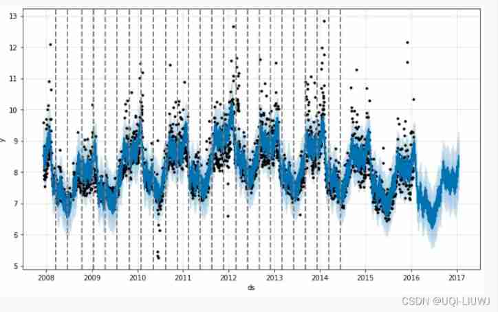
Although there are many places where we may change the trend , But because the priors are sparse , Most of these change points are not used . We can see this by plotting the rate change amplitude of each change point :

The location of significant change points can be visualized in the following ways :( Here is the linear trend prophet)
plot(m,forecast)+add_changepoints_to_plot(m)

By default , Only the first of the time series 80% Infer the point of change , In order to have enough time segments to predict future trends and avoid over fitting fluctuations at the end of the time series .
This default value applies to many situations , But not all . have access to changepoint_range Parameter changes .
m <- prophet(changepoint.range = 0.9)
3.2 Flexibility to adjust trend changes
If the trend changes too well ( Too much flexibility ) Or under fitting ( Lack of flexibility ), You can use input parameters changepoint_prior_scale Adjust the intensity of the sparse prior .
By default , This parameter is set to 0.05
Adding it will make the trend more flexible
m <- prophet(df, changepoint.prior.scale = 0.5)
You can find , Compared with the previous situation , There are many changes here , At the same time, the range has also increased

Reducing it will become inflexible
m <- prophet(df, changepoint.prior.scale = 0.001)

3.3 Manually specify the location of the change point
have access to changepoints Parameters manually specify the location of potential change points , Instead of using automatic change point detection . Then it will only be allowed to change the slope at these points , And use the same sparse regularization as before .
m <- prophet(df,changepoints = c('2014-01-01','2010-02-03')) 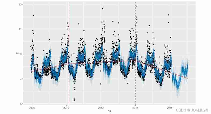
4 The holiday season
4.1 Provide holidays manually
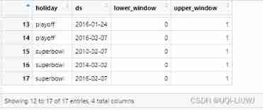
If you have holidays or other special events that you want to model , You must create a data frame for them . It has two columns (holiday and ds), Every holiday has a line .
All events of the holiday must be included , Including the past ( In terms of historical data ) And the future ( In terms of prediction ).
If they don't repeat in the future ,Prophet They will be modeled , Then don't include them in the forecast .
You can also include columns lower_window and upper_window , They extend their holidays to around [lower_window, upper_window] God .
library(dplyr)

playoffs <- data_frame(
  holiday = 'playoff',
  ds = as.Date(c('2008-01-13', '2009-01-03', '2010-01-16',
                 '2010-01-24', '2010-02-07', '2011-01-08',
                 '2013-01-12', '2014-01-12', '2014-01-19',
                 '2014-02-02', '2015-01-11', '2016-01-17',
                 '2016-01-24', '2016-02-07')),
  lower_window = 0,
  upper_window = 1
)
# The holiday is extended to one day after the date


superbowls <- data_frame(
  holiday = 'superbowl',
  ds = as.Date(c('2010-02-07', '2014-02-02', '2016-02-07')),
  lower_window = 1,
  upper_window = 0
)
# The holiday is extended to the day before the date

holidays <- bind_rows(playoffs, superbowls)
establish holiday After the table , By using holidays Parameters include holiday effects in the forecast .
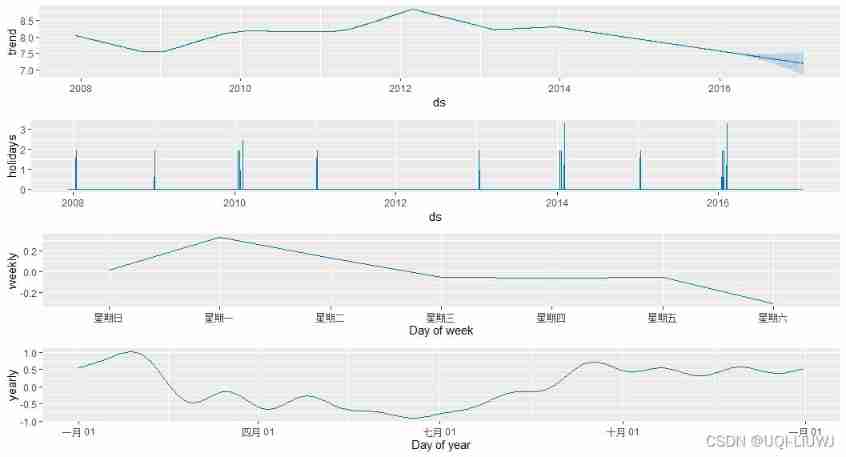
m <- prophet(df,holidays = holidays)

forecast <- predict(m, future)

prophet_plot_components(m,forecast)
Compared with before , There are more holiday Influence
You can use a method similar to sql The way see holiday Influence
forecast %>%
  select(ds, playoff, superbowl) %>%
  filter(abs(playoff + superbowl) > 0)


          ds  playoff superbowl
1  2008-01-13 1.220577  0.000000
2  2008-01-14 1.909146  0.000000
3  2009-01-03 1.220577  0.000000
4  2009-01-04 1.909146  0.000000
5  2010-01-16 1.220577  0.000000
6  2010-01-17 1.909146  0.000000
7  2010-01-25 1.909146  0.000000
8  2010-02-07 1.220577  1.215571
9  2011-01-08 1.220577  0.000000
10 2011-01-09 1.909146  0.000000
11 2013-01-12 1.220577  0.000000
12 2013-01-13 1.909146  0.000000
13 2014-01-12 1.220577  0.000000
14 2014-01-13 1.909146  0.000000
15 2014-01-19 1.220577  0.000000
16 2014-01-20 1.909146  0.000000
17 2014-02-02 1.220577  1.215571
18 2014-02-03 1.909146  1.384333
19 2015-01-11 1.220577  0.000000
20 2015-01-12 1.909146  0.000000
21 2016-01-17 1.220577  0.000000
22 2016-01-18 1.909146  0.000000
23 2016-01-24 1.220577  0.000000
24 2016-01-25 1.909146  0.000000
25 2016-02-07 1.220577  1.215571
26 2016-02-08 1.909146  1.384333
4.2 Provide national holidays
You can use add_country_holidays Method uses the built-in country specific / Regional holiday collection .
Designated country / The name of the region , Then in addition to passing 4.1 Outside any designated holidays , It will also include the country / Major holidays in the region :
But here is one thing to explain , stay add_country_holidays Before , You can't fit model, For example, the following code , You're going to report a mistake
m <- prophet(df,holidays = holidays)

m<-add_country_holidays(m,'US')

#Error in add_country_holidays(m, "China") :
#  Country holidays must be added prior to model fitting.
m <- prophet(holidays = holidays)

m<-add_country_holidays(m,'CN')

m<-fit.prophet(m,df)

forecast <- predict(m, future)

prophet_plot_components(m,forecast)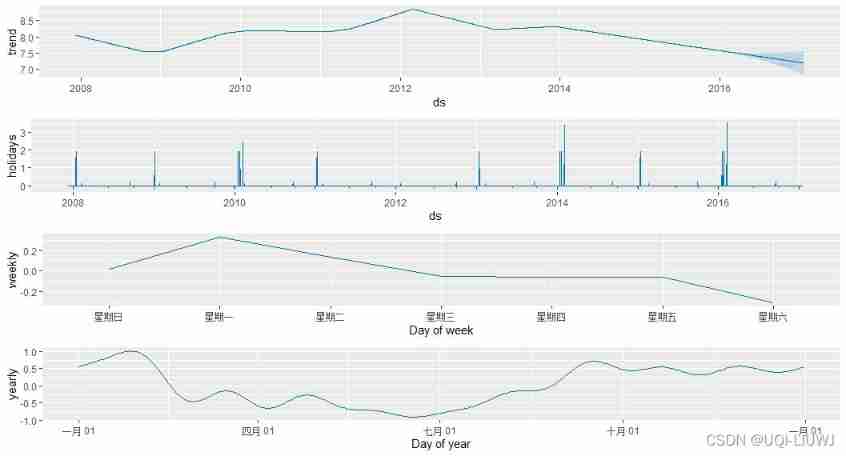
4.2.1 View the currently set holidays
Add observed It means that there is only in the observation set
m$train.holiday.names
[1] "playoff"              "superbowl"            "New Year's Day"       "Chinese New Year"
[5] "Tomb-Sweeping Day"    "Labor Day"            "Dragon Boat Festival" "Mid-Autumn Festival"
[9] "National Day"
4.2.2 National holidays available
Available countries / List of regions and countries to use / The name of the region can be found on its page :https://github.com/dr-prodigy/python-holidays.
Except for these countries / region ,Prophet It also includes the following countries / Holidays in the region : Brazil (BR)、 Indonesia (ID)、 India (IN)、 Malaysia (MY)、 Vietnam (VN)、 Thailand (TH)、 the Philippines (PH)、 Pakistan ( PK)、 Bangladesh (BD)、 Egypt (EG)、 China (CN)、 Russia (RU)、 South Korea (KR)、 belarus (BY) And the United Arab Emirates (AE).
stay R in , The holiday date is from 1995 Year to 2044 Annual , And as a data-raw/generated_holidays.csv Stored in the package .
4.3 Holiday scale
If you find that the holiday is too fitting , You can use parameters holiday_prior_scale Adjust its prior scale to make it smooth .
By default , This parameter is 10, It provides very little regularization . Reducing this parameter will weaken the holiday effect , Increase will emphasize the role of holidays :
m <- prophet(df, holidays = holidays, holidays.prior.scale = 1000)5 Seasonality
5.1 Seasonal Fourier series
Use the sum of partial Fourier series to estimate seasonality
partial sums ( The order ) The number of items in is a parameter that determines the rate of seasonal change .
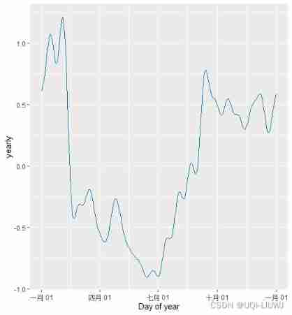
The default Fourier order for annual seasonality is 10
m <- prophet(df)
prophet:::plot_yearly(m)

The default value is usually appropriate , But when seasonality needs to adapt to higher frequency changes, they can be increased , And usually not very smooth . When instantiating the model , Fourier order can be specified for each built-in seasonal , Add here to 20:
Increasing the number of Fourier terms can make seasonality adapt to faster change cycles , But it can also lead to over fitting :N Fourier terms correspond to 2N A variable
m <- prophet(df, yearly.seasonality = 20)
prophet:::plot_yearly(m)
5.2 Specify custom seasonality
If the length of the time series exceeds two cycles ,Prophet The weekly and annual seasonality will be fitted by default .
have access to add_seasonality Method 、 Add other seasonality ( monthly 、 Quarterly 、 Every hour ).
The input to this function is the name 、 Seasonal cycle ( In days ) And seasonal Fourier order . As a reference ,Prophet By default 3 rank Fourier order It means weekly seasonality ,10 Indicates annual seasonality .
Here and add_country_holidays equally , You can't fit first
 m<-prophet()
 m<-add_seasonality(m, name='monthly', period=30.5, fourier.order=5)
 m<-fit.prophet(m,df)
 forecast <- predict(m, future)
prophet_plot_components(m, forecast) 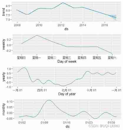
5.3 Cancel a certain seasonality
m<-prophet(df,weekly.seasonality = FALSE)
forecast <- predict(m, future)
prophet_plot_components(m, forecast)
5.4 Depending on the seasonality of other factors
In some cases , Seasonality may depend on other factors , For example, the seasonal pattern of each week in summer is different from the rest of the year , Or a daily seasonal pattern that differs between weekends and weekdays . These types of seasonality can be modeled using conditional seasonality .
The default weekly seasonality assumes that the pattern of weekly seasonality throughout the year is the same , But we expect the weekly seasonal pattern in the peak season 、 It's different from the off-season . We can use conditional seasonality to construct separate weekly seasonality in peak season and off season .
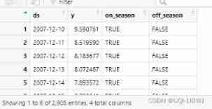
First , We add a Boolean column to the data frame , Indicate whether each date is in the peak season or the off-season :
is_nfl_season <- function(ds) {
  dates <- as.Date(ds)
  #  Each element is similar to "2016-01-15"
  month <- as.numeric(format(dates, '%m'))
  # format(dates, '%m') Returns the month of character type
  # as.numeric Convert to numbers
  return(month > 8 | month < 2)
}

# Declare a function , If in 8 After month , Two months ago , That's it True, It is False
df$on_season <- is_nfl_season(df$ds) df$off_season <- !is_nfl_season(df$ds)
Then we disable the built-in weekly seasonality , And replace it with two weekly Seasonalities that specify these columns as conditions .
This means that seasonality only applies to condition_name As a True Date .
We must also add this column to the future data frame we are predicting .
m <- prophet(weekly.seasonality=FALSE)
m <- add_seasonality(m,
                    name='weekly_on_season',
                    period=7,
                    fourier.order=3,
                    condition.name='on_season')
m <- add_seasonality(m,
                    name='weekly_off_season',
                    period=7,
                    fourier.order=3,
                    condition.name='off_season')
m <- fit.prophet(m, df)

future$on_season <- is_nfl_season(future$ds)
future$off_season <- !is_nfl_season(future$ds)
forecast <- predict(m, future)
prophet_plot_components(m, forecast)
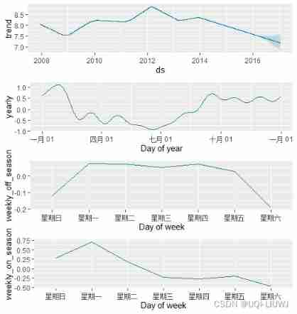
Now? , Both seasonality are shown in the component diagram above . We can see , During peak season , There is a sharp increase on Sunday and Monday , In the off-season, there is no .
5.5 Specify seasonal scale
Like holidays , Seasonality also has a scale seasonality_prior_scale
m <- add_seasonality(
    m,
    name='weekly',
    period=7,
    fourier.order=3,
    prior.scale=0.1)
6 Multiplicative seasonality
By default ,Prophet Fitting addition seasonality , This means adding seasonal influences to the trend to get predictions
Let's look at a situation , As shown in the figure below , This time series has an obvious annual cycle , But the predicted seasonality is too large at the beginning and too small at the end of the time series . In this time series , Seasonality is not Prophet Assumed constant addition factor , It grows with the trend . This is seasonal multiplication .

Prophet You can set seasonality_mode='multiplicative' To fit the seasonality of multiplication :
m <- prophet(df, seasonality.mode = 'multiplicative')Use seasonality_mode='multiplicative', The holiday effect will also be modeled as multiplication .
By default , Any added seasonality will be set to seasonality_mode, But you can specify mode='additive' or mode='multiplicative' Override... As a parameter
m <- prophet(seasonality.mode = 'multiplicative')
m <- add_seasonality(m,
                    'quarterly',
                    period = 91.25,
                    fourier.order = 8,
                    mode = 'additive')
7 Uncertainty interval
By default ,Prophet The forecast will be returned yhat The uncertainty interval of .
There are three uncertainty intervals in the prediction : The uncertainty of the trend 、 Seasonal estimation uncertainty and additional observation noise .
7.1 The uncertainty of the trend
The biggest source of uncertainty in the forecast is the possibility of future trend changes . We assume that we will see similar trend changes in the future . especially , We assume that the average frequency and amplitude of future trend changes will be the same as what we have observed in history . We predict these trends ahead , And by calculating their distribution , We get the uncertainty interval .
A characteristic of this way of measuring uncertainty is , By increasing the changepoint_prior_scale To allow prediction to have a larger desirable range , Increase the uncertainty of the forecast .
You can use parameters interval_width Set the width of the uncertain interval ( The default is 80%):
m <- prophet(df, interval.width = 0.95)
forecast <- predict(m, future)
plot(m,forecast)
Compared with before , The uncertainty range is larger
7.2 Seasonal uncertainty
By default ,Prophet Only the uncertainty of trend and observation noise will be returned . To get seasonal uncertainty , Complete Bayesian sampling must be carried out . This is the use of parameters mcmc.samples( The default is 0) Accomplished .
m <- prophet(df, mcmc.samples = 300)
forecast <- predict(m, future)
It works MCMC Sampling replaces the typical MAP It is estimated that , And it may take longer , It depends on how many observations - Expect minutes, not seconds .
When plotting seasonal components , You will see their uncertainty :
prophet_plot_components(m,forecast)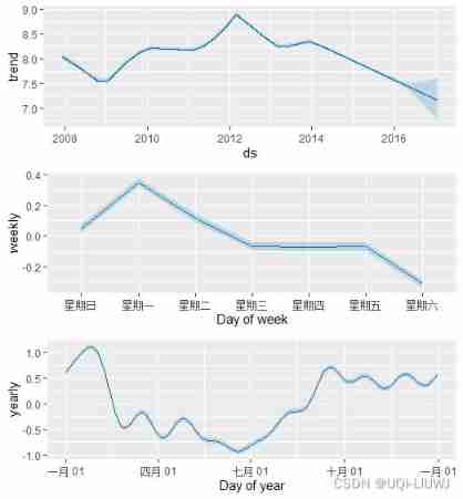
8 outliers
Outliers can affect... In two main ways Prophet The forecast . ad locum , We're right about what we recorded before R Page Wikipedia The visit was predicted , But there is a bad data block :
df<-read.csv('C:/Users/16000/example_wp_log_R_outliers1.csv')
m <- prophet(df)
future <- make_future_dataframe(m, periods = 1096)
forecast <- predict(m, future)
plot(m, forecast) 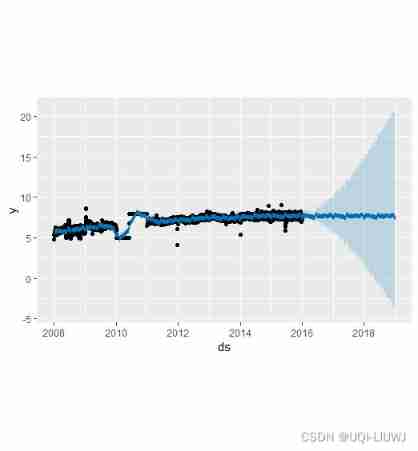
The trend forecast seems reasonable , But the uncertainty range seems too wide . Prophet Able to handle outliers in history , But only by matching them to trends . then , The uncertainty model predicts future trend changes of similar magnitude .
The best way to handle outliers is to delete them ——Prophet There is no problem with missing data . If you set their values to NA But keep the date in the future , that Prophet Will give you a prediction of their values .
outliers <- (as.Date(df$ds) > as.Date('2010-01-01')
             & as.Date(df$ds) < as.Date('2011-01-01'))
df$y[outliers] = NA
m <- prophet(df)
forecast <- predict(m, future)
plot(m, forecast)
After removing outliers , The trend is the same as when the outliers were not removed , But the uncertainty range is much smaller
9 Non daily data
Prophet It can be done by ds The data frame with timestamp is passed in the column to predict the time series of non daily data . The timestamp format should be YYYY-MM-DD HH:MM:SS .

ad locum , We will Prophet Fit to 5 Minutes is the frequency data :
df<-read.csv('C:/Users/16000/example_yosemite_temps.csv')

m <- prophet(df)

future <- make_future_dataframe(m, periods = 300, freq = 60 * 60)
# first 60 It means a few minutes , the second 60 For seconds  ( The product represents the number of seconds between each two prediction intervals )

fcst <- predict(m, future)
plot(m, fcst)
(freq= This can also be a string, such as “month” such )

At this point, we draw the graph after time series decomposition ,daily seasonality It has become seasonal at different times
prophet_plot_components(m,fcst)
边栏推荐
- KS008基于SSM的新闻发布系统
- 10個 Istio 流量管理 最常用的例子,你知道幾個?
- 阿里测试师用UI自动化测试实现元素定位
- How to modify field constraints (type, default, null, etc.) in a table
- DM8 backup set deletion
- The Research Report "2022 RPA supplier strength matrix analysis of China's banking industry" was officially launched
- Custom event of C (31)
- Mathematical modeling regression analysis relationship between variables
- Cf603e pastoral oddities [CDQ divide and conquer, revocable and search set]
- Global and Chinese market of aircraft anti icing and rain protection systems 2022-2028: Research Report on technology, participants, trends, market size and share
猜你喜欢

C#(二十八)之C#鼠标事件、键盘事件

lora网关以太网传输
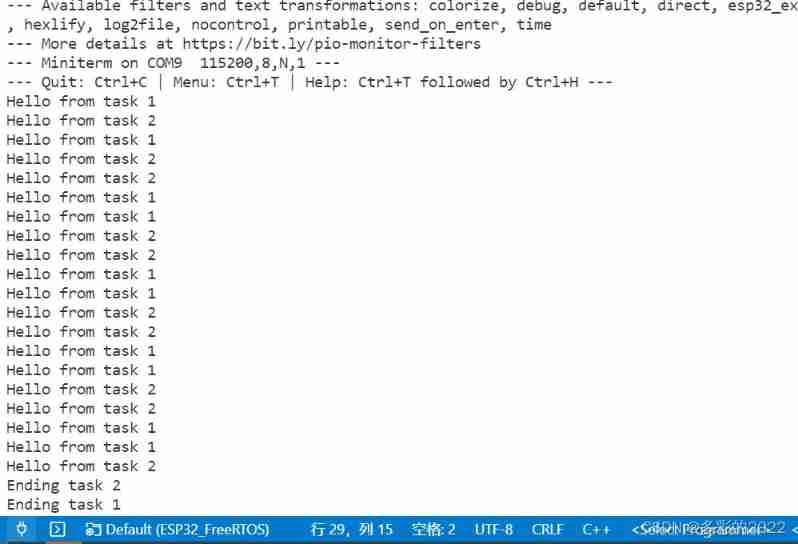
ESP32_ FreeRTOS_ Arduino_ 1_ Create task

Web components series (VII) -- life cycle of custom components

Simple blog system
【PSO】基于PSO粒子群优化的物料点货物运输成本最低值计算matlab仿真,包括运输费用、代理人转换费用、运输方式转化费用和时间惩罚费用

Facebook and other large companies have leaked more than one billion user data, and it is time to pay attention to did
在 .NET 6 中使用 Startup.cs 更简洁的方法

Stack and queue

综合能力测评系统
随机推荐
Use js to complete an LRU cache
C language -- structs, unions, enumerations, and custom types
Basic knowledge of binary tree, BFC, DFS
pd. to_ numeric
2/11 matrix fast power +dp+ bisection
math_ Derivative function derivation of limit & differential & derivative & derivative / logarithmic function (derivative definition limit method) / derivative formula derivation of exponential functi
C form application of C (27)
Benefits of automated testing
【FPGA教程案例11】基于vivado核的除法器设计与实现
Fundamentals of SQL database operation
Redis (replicate dictionary server) cache
C#(三十)之C#comboBox ListView treeView
IDEA编译JSP页面生成的class文件路径
绑定在游戏对象上的脚本的执行顺序
[Zhao Yuqiang] deploy kubernetes cluster with binary package
Brief tutorial for soft exam system architecture designer | general catalog
C#(二十九)之C#listBox checkedlistbox imagelist
Oracle ORA error message
Cf464e the classic problem [shortest path, chairman tree]
Global and Chinese markets for fire resistant conveyor belts 2022-2028: Research Report on technology, participants, trends, market size and share