[beauty of algebra] singular value decomposition (SVD) and its application to linear least squares solution ax=b

Singular value decomposition （Singular Value Decomposition,SVD） Is an important matrix decomposition in linear algebra , Is the generalization of eigen decomposition on any matrix , In stereo vision 、 3D reconstruction is widely used . Because it can be used to solve the least square solution of linear equations , So in solving the essential matrix 、 Homography matrix 、 Point cloud rigid transformation matrix , Can use SVD. This article will give you a brief introduction to singular value decomposition , And through formula derivation to explain its application in linear least square solution $Ax=b$ Application on .

Singular value decomposition （SVD Decomposition） Definition

For any matrix $A\in R^{m\times n}$, There are orthogonal matrices $U\in R^{m\times m}$,$V\in R^{n\times n}$, And diagonal matrix $\Sigma \in R^{m\times n}$：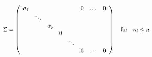


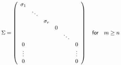
among , Diagonal elements meet ：
$${\sigma }_1\ge \cdots \ge {\sigma }_r\ge {\sigma }_{r+1}=\cdots ={\sigma }_{\min (m,n)}=0$$
bring ,$A=U\Sigma V^T$.

This decomposition is called matrix $A$ Singular value decomposition of （Singular Value Decomposition）, Is a very important matrix decomposition , Diagonal matrix $\Sigma$ Diagonal elements of ${\sigma }_i$ Called matrix $A$ The singular value of . matrix $U$ The column vector of becomes a left singular vector , matrix $V$ The column vector of becomes a right singular vector .

Use orthogonal matrix $V$, The following formula can be obtained ：
$$AV=U\Sigma$$

This can be explained as , There is a special set of orthogonal vectors （ for example $V$ Column vector set of ）, Through the matrix $A$ Map to another set of orthogonal vectors （ for example $U$ Column vector set of ）.

SVD Some characteristics of

Given matrix $A$ A group of SVD decompose
$$A=U\Sigma V^T$$

among ,${\sigma }_1\ge \cdots \ge {\sigma }_r\ge {\sigma }_{r+1}=\cdots ={\sigma }_{\min (m,n)}=0$

There is a corollary （$R(A)$ and $N(A)$ They are matrices $A$ Range space and zero space ）：

• $rank(A)=r$
• $R(A)=R([u_1,...u_r])$
• $N(A)=R([u_{r+1},...,u_n])$
• $R(A^T)=R([v_1,...v_r])$
• $N(A^T)=R([v_{r+1},...,v_m])$

If we introduce
$$U_r=[u_1,...,u_r],\Sigma =diag({\sigma }_1,...,{\sigma }_r),V_r=[v_1,...,v_r]$$

Then there are
$$A=U_r{\Sigma }_r{V}_r^T=\sum _{i=1}^r{\sigma }_i{u}_i{v}_i^T$$
This is called a matrix $A$ Binary decomposition of （dyadic decomposition）, About to rank as $r$ Matrix $A$ Decompose into $r$ One rank is 1 Sum of matrices .

meanwhile , You can get
$$A^{T}A=V{\Sigma }^T\Sigma V^{T}andA{A}^T=U\Sigma {\Sigma }^T{U}^T$$

You know , Square of singular value ${\sigma }_i^2,i=1,...,p$ It's a symmetric matrix $A^{T}A$ and $A{A}^T$ The eigenvalues of the ,$v_i$ and $u_i$ They are the corresponding eigenvectors . The proof is as follows ：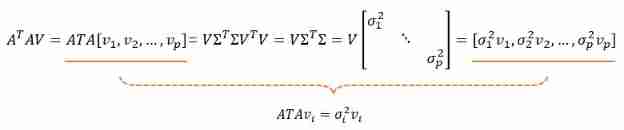

This conclusion is very useful , We are trying to understand $Ax=0$ when , Requirements $A^{T}A$ The eigenvector corresponding to the minimum eigenvalue of , That is to say SVD Decomposed matrix $V$ The last column of . Another application scenario is the covariance matrix PCA When analyzing , You can use SVD Decomposed matrix $V$ Each column is a vector in each direction .

Through this conclusion , We can easily calculate the matrix $A$ Of 2- Norm sum Frobenius norm ：
$$\begin{array}{rl}||A|{|}_2& =\sqrt{\underset{x\ne 0}{\max }\frac{||Ax|{|}_2}{||x|{|}_2}}=\sqrt{\underset{x\ne 0}{\max }\frac{x^T{A}^{T}Ax}{x^{T}x}}=\sqrt{\underset{x\ne 0}{\max }\frac{x^T{\lambda }_{A^{T}A}x}{x^{T}x}}=\sqrt{\underset{x\ne 0}{\max }{\lambda }_{A^{T}A}}={\sigma }_1\\ ||A|{|}_F& =\sqrt{\sum _{i=1}^m\sum _{j=1}^n{a}_{ij}^2}=\sqrt{trace(A^{T}A)}=\sqrt{{\sigma }_1^2+\cdots +{\sigma }_p^2},p=\min (m,n)\end{array}$$

SVD Solve the linear least square problem Ax=b

Let's see SVD The classic application of ： Solve the least square solution of linear equation .

Consider a linear least squares problem $Ax=b$：
$$\underset{x}{\min }||Ax-b|{|}_2^2$$

Given matrix $A\in R^{m\times n}$ A group of SVD decompose ：$A=U\Sigma V^T$

According to the matrix $U$ and $V$ The orthogonality of , Yes
$$||Ax-b|{|}_2^2=||U^T(Ax-b)|{|}_2^2=||U^{T}Ax-U^{T}b|{|}_2^2=||\Sigma V^{T}x-U^{T}b|{|}_2^2$$

another $z=V^{T}x$, Then there are
$$||Ax-b|{|}_2^2=||\Sigma V^{T}x-U^{T}b|{|}_2^2=\sum _{i=1}^r({\sigma }_i{z}_i-u_i^{T}b{)}^2+\sum _{i=r+1}^m(u_i^{T}b{)}^2$$

therefore ,
$$\underset{x}{\min }||Ax-b|{|}_2^2=\underset{x}{\min }(\sum _{i=1}^r({\sigma }_i{z}_i-u_i^{T}b{)}^2+\sum _{i=r+1}^m(u_i^{T}b{)}^2)$$

obviously , When ${\sigma }_i{z}_i=u_i^{T}b$ when , Take the minimum , Then the least square solution is ：
$$\begin{array}{rl}{z}_i& =\frac{u_i^{T}b}{{\sigma }_i},i=1,...,r\\ z_i& =arbitrary,i=r+1,...,n\end{array}$$

The minimum value is
$$\underset{x}{\min }||Ax-b|{|}_2^2=\sum _{i=r+1}^m(u_i^{T}b{)}^2$$

from $z=V^{T}x$, Available $x=Vz$, therefore , adopt SVD The formula for finding the linear least square solution is
$$\begin{array}{rl}x& =Vz\\ z_i& =\frac{u_i^{T}b}{{\sigma }_i},i=1,...,r\\ z_i& =arbitrary,i=r+1,...,n\end{array}$$

In the above formula, we find , When $r=n$ when , There is a unique least square solution , When $r<n$ when , There are countless least squares solutions , At this point, we can find the minimum norm solution ：
$$\begin{array}{rl}{x}_{†}& =V{z}_{†}\\ z_i^{†}& =\frac{u_i^{T}b}{{\sigma }_i},i=1,...,r\\ z_i^{†}& =0,i=r+1,...,n\end{array}$$

We know that the least square solution can also pass $(A^{T}A{)}^{-1}(A^{T}b)$ To solve , And by SVD The advantage of the solution is that it does not need complex inverse operation , And can handle $A^{T}A$ It is the case that the singular matrix is irreversible .

About bloggers ：
Ethan Li Li Yingsong （ You know ： Li Yingsong ）
Wuhan University Doctor of photogrammetry and remote sensing

Main direction Stereo matching 、 Three dimensional reconstruction

2019 Won the first prize of scientific and technological progress in surveying and mapping in （ Provincial and ministerial level ）

Love 3D , Love sharing , Love open source
GitHub： https://github.com/ethan-li-coding
mailbox ：[email protected]

Personal wechat ：

Welcome to exchange ！

Pay attention to bloggers and don't get lost , thank ！
Blog home page ：https://ethanli.blog.csdn.net