当前位置：网站首页>[Clickhouse kernel principle graphic explanation] about the collaborative work of partitioning, indexing, marking and compressed data

[Clickhouse kernel principle graphic explanation] about the collaborative work of partitioning, indexing, marking and compressed data

2022-07-06 12:23:00 【Donghai Chen Guangjian】

summary

ClickHouse It's an on-line analytical process （OLAP） Column database management system （Columnar DBMS）.

Partition 、 Indexes 、 Marking and compressing data , These components work together to ClickHouse Database brings very efficient query performance .

Everything is a mapping . Lightsaber

This article first briefly introduces these components . Then, from the writing process 、 The query process , And three corresponding relations between data mark and compressed data block .

Partition 、 Indexes 、 Introduction to the core components of marking and compressing data

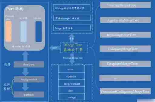
MergeTree Engine storage structure

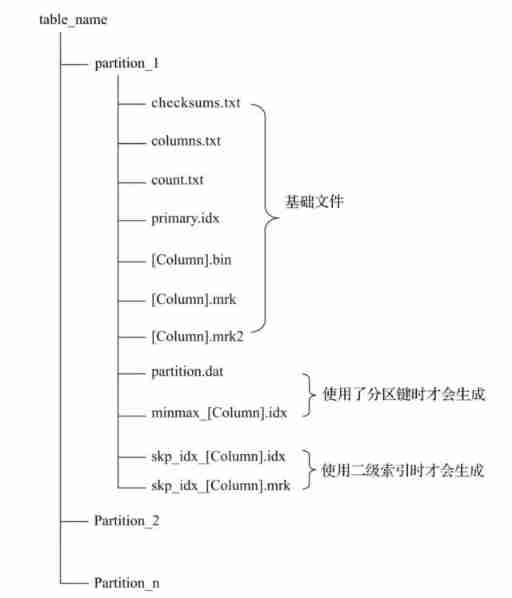
MergeTree Storage structure of

partition： Partition Directory , The remaining data files （primary.idx、[Column].mrk、[Column]. bin etc. ） Are organized and stored in the form of partition directories , Data belonging to the same partition , It will eventually be merged into the same partition Directory , Data from different partitions , Will never be merged .
checksums： Verify File , Store in binary format . It saves the rest of the files (primary. idx、count.txt etc. ) Of size Size and size Hash value of , It is used to quickly verify the integrity and correctness of files .
columns.txt： Column information file , Store in clear text format , Used to save the column field information under this data partition .
count.txt： Count files , Store in clear text format , Used to record the total number of rows of data under the current data partition directory .
primary.idx： First level index file , Store in binary format . Used to store sparse indexes , a sheet MergeTree A table can only declare a first level index once . With sparse index , When querying data, data files outside the range of primary key conditions can be excluded , So as to effectively reduce the data scanning range , Speed up query .
[Column].bin： Data files , Store in a compressed format , Used to store data in a column . because MergeTree Use column storage , So each column field has its own .bin Data files , And name it with the column field name .
[Column].mrk： Store in binary format . The tag file contains .bin Offset information of data in the file . Mark file alignment with sparse index , And .bin The documents correspond to each other , therefore MergeTree Created by marking files primary.idx Sparse index and .bin Mapping between data files . That is, first through sparse index （primary.idx） Find the offset information of the corresponding data （.mrk）, Then directly from... By offset .bin The data is read from the file . because .mrk Tag files with .bin The documents correspond to each other , therefore MergeTree Each column field in the has its corresponding .mrk Tag file
[Column].mrk2： If an index interval of adaptive size is used , The tag file will be marked with ．mrk2 name . Its working principle and function are similar to ．mrk The tag file is the same .
partition.dat And minmax_[Column].idx： If the partition key is used , for example PARTITION BY EventTime, Will generate additional partition.dat And minmax Index file , They are stored in binary format .partition.dat Used to save the final value generated by the partition expression under the current partition ; and minmax The index is used to record the minimum and maximum values of the partition field corresponding to the original data under the current partition .
skp_idx_[Column].idx And skp_idx_[Column].mrk： If the secondary index is declared in the table building statement , The corresponding secondary index and tag files will be generated additionally , They also use binary storage . The secondary index is in ClickHouse Also known as hop index .

Partition

stay MergeTree in , Data is organized in the form of partitioned directories , Each partition is stored separately : Partition_1, Partition_2, Partition_3, Partition_4, .....

With this form , In the face of MergeTree When making data query , It can effectively skip useless data files , Use only the smallest subset of partitioned directories .

Partition rules of data

MergeTree The rules for data partitioning are defined by the partition ID decision , Specific to each data partition ID, Is determined by the value of the partition key . Partitioning keys support the declaration of... Using any one or a set of field expressions , Its business semantics can be years 、 month 、 Any rule such as day or organizational unit . According to different value data types , Partition ID The generation logic currently has four rules ：

（1） Do not specify partition key ： If you don't use the partition key , I don't use PARTITION BY Declare any partition expression , Then partition ID The default name is all, All data will be written to this all Partition .
（2） Use integer ： If the partition key value belongs to integer ( compatible UInt64, It includes signed integers and unsigned integers ), And cannot be converted to date type YYYYMMDD Format , Then output directly in the character form of the integer , As a partition ID The value of .
（3） Use date type ： If the partition key value belongs to the date type , Or it can be transformed into YYYYMMDD Integer of format , Use according to YYYYMMDD Output in the form of formatted characters , And as a partition ID The value of .
（4） Use other types ： If the partition key value is not an integer , It's not a date type , for example String、Float etc. , Through 128 position Hash The algorithm takes its Hash Value as partition ID The value of . When data is written , Will compare the partition ID Fall into the corresponding data partition

partition： Partition Directory , All kinds of data files inside （primary.idx、data.mrk、data.bin wait ） Are organized and stored in the form of partition directories , Data belonging to the same partition , It will eventually be merged into the same partition Directory , Data from different partitions will never be merged .

The naming rule of partition directory is ：PartitionID_MinBlockNum_MaxBlockNum_Level

Let's explain these parts ：

1）PartitionID： Partition ID, There should be no need to say more about this .

2）MinBlockNum、MaxBlockNum： Minimum block number and maximum block number , The naming here is easily reminiscent of the data compression block to be mentioned later , Even cause confusion , But in fact, there is no relationship between the two . there BlockNum It's a self increasing integer , from 1 Start , Every time a new partition is created, it will grow by itself 1, And for a new partition directory , its MinBlockNum and MaxBlockNum They are equal. . such as 202005_1_1_0、202006_2_2_0、202007_3_3_0, And so on . But there are exceptions , When the partition directory is merged , So MinBlockNum and MaxBlockNum There will be other rules , Let's talk about it later .

3）Level： The level of consolidation , It can be understood as the number of times a partition is merged , there Level and BlockNum Different , It is not globally cumulative . For each newly created directory , Their initial values are 0, Then, take the partition as the unit , If the same partition is merged , Then the partition corresponds to Level Add 1. Maybe some people don't understand here " Merge the same partition " What does it mean , Let's introduce .

The merging process of partition directories

MergeTree The partition directory of is different from other traditional databases , First MergeTree The partition directory does not exist after the data table is created , It is created in the process of data writing , If there is no data in a table , Then there will be no partition directory . It's easy to understand , Because the name of partition directory and partition ID of , And zoning ID It is also related to the value corresponding to the partition key , And there is not even data in the table , So how to partition directories .

secondly ,MergeTree The partition directory of is not immutable , In the design of other databases , When adding data, the directory itself will not change , Just append data files in the same partition . and MergeTree Completely different , With every write of data ,MergeTree Will generate a batch of new partition directories , Even if the data written in different batches belong to the same partition , Different partition directories will also be generated . That is to say, for the same partition , There will be cases corresponding to multiple partition directories . And then at some point （ commonly 10 To 15 minute ）,ClickHouse Multiple directories belonging to the same partition will be merged through background tasks （Merge） Into a new directory , Of course, it can also be optimize TABLE table_name FINAL Statements merge immediately , As for the old directory before the merger, it will be at some time later （ Default 8 minute ） Be deleted .

Multiple directories belonging to the same partition , After merging, a new directory will be generated , The indexes and data files in the directory are merged accordingly . The name of the new directory is generated according to the following rules ：

1.PartitionID： unchanged
2.MinBlockNum： Take the smallest of all directories in the same partition MinBlockNum
3.MaxBlockNum： Take the largest of all directories in the same partition MaxBlockNum
4.Level： Take the maximum in the same partition Level Value plus 1

There is one thing that needs to be made clear , stay ClickHouse in , Data partition （partition） And data slicing （shard） It's a completely different concept . Data partitioning is for local data , It is a vertical segmentation of data .MergeTree You can't rely on the characteristics of partitions , Distribute the data of a table to multiple ClickHouse Service node . Horizontal segmentation is data segmentation （shard） The ability of .

Indexes

First level index

primary.idx： First level index file , Store in binary format , Used to store sparse indexes , a sheet MergeTree A table can only declare a first level index once （ adopt ORDER BY or PRIMARY KEY）. With sparse index , When querying data, data files outside the range of primary key conditions can be excluded , So as to effectively reduce the data scanning range , Speed up query .

The bottom layer of the first level index adopts sparse indexing , From the figure below, we can see the difference between it and dense index .

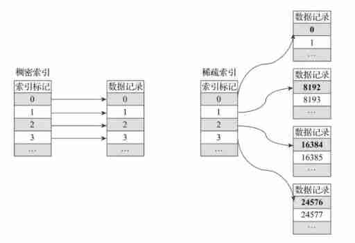
Comparison diagram of sparse index and dense index

For dense indexes , Each row of index marks will correspond to a specific row of records . In sparse indexes , Each row of index marks a large piece of data , Not a specific line （ The difference between them is a little similar mysql in innodb Clustered index and nonclustered index of ）.

The advantages of sparse indexing are obvious , It only needs a few index marks to record the interval location information of a large amount of data , And the greater the amount of data, the more obvious the advantage . For example, we use the default index granularity （8192） when ,MergeTree It only needs 12208 The row index mark can be 1 100 million rows of data records provide an index . Because sparse index takes up less space , therefore primary.idx The index data in can be resident in memory , The access speed is naturally very fast .

Index granularity index_granularity

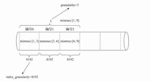
Index granularity is like a ruler , Will measure the length of the entire data , And mark the data according to the scale , Finally, the data is marked into small segments with multiple intervals . The data to index_granularity Granularity ( The old version defaults to 8192, The new version realizes adaptive granularity ) Marked as multiple small intervals , Each interval has a maximum of 8192 Row data ,MergeTree Use MarkRange Represents a specific interval , And pass start and end Indicates its specific scope . As shown in the figure below .

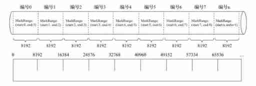
Index granularity is when creating tables , stay SETTINGS Specify the inside index_granularity The control of the , although ClickHouse Provides the feature of adaptive granularity , But for ease of understanding , We will introduce it with fixed index granularity （8192）. Index granularity for MergeTree Is a very important concept , It is like a ruler , Will measure the length of the entire data , And mark the data according to the scale , Finally, the data is marked into small segments with multiple intervals .

The data to index_granularity Granularity （ Default 8192） Marked as multiple small intervals , Each interval has a maximum of 8192 Row data ,MergeTree Use MarkRange Represents a specific interval , And pass start and end Indicates its specific scope .index_granularity Although the name of takes the word index , But it does not only work on primary indexes , It will also affect the data mark file （data.mrk） And data files （data.bin）. Because only the first level index cannot complete the query , It needs the offset in the tag file to locate the data , Therefore, the interval granularity of primary index and data mark （ A fellow index_granularity That's ok ） identical , Align with each other , And the data file will also follow index_granularity The interval granularity of generates compressed data blocks .

Secondary indexes

skp_idx_[IndexName].idx and skp_idx_[IndexName].mrk3： If the secondary index is specified in the table creation statement , The corresponding secondary index file and tag file will be generated additionally , They also use binary storage . The secondary index is in ClickHouse Is also called hop index , Currently owned minmax、set、ngrambf_v1 and token_v1 Four types , The purpose of these kinds of hop index is the same as that of primary index , Is to further reduce the scanning range of data , So as to speed up the whole query process .

Mark

If you put MergeTree Compared to a Book ,primary.idx The primary index is like the primary chapter catalogue of this book ,.bin The data in the document is like the text in this book , So the data tag (.mrk) The association will be established between the first level chapter directory and the specific text ( Bookmarks ). For data markers , It records two important information ：

firstly , It is the page information corresponding to the first level chapter ;

second , It is the starting position information of a paragraph of text on a page .

thus , Through data markers, you can quickly turn from a book to the page where you pay attention to the content , And know which line to start reading .

data.mrk： Tag file

Store in binary format , The tag file contains data.bin Offset information of data in the file , And the mark file is aligned with the sparse index , therefore MergeTree A sparse index is established by marking the file （primary.idx） And data files （data.bin） Mapping between . And when reading data , First, through sparse index （primary.idx） Find the offset information of the corresponding data （data.mrk）, Because the two are aligned , Then, according to the offset information, directly from data.bin The data is read from the file .

data.mrk3： If an index interval of adaptive size is used , The tag file will be marked with data.mrk3 ending , But its working principle is similar to data.mrk The files are the same .

Data tags serve as a bridge between primary indexes and data , It's like a bookmark , And every chapter of the book always has its own bookmark .

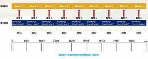
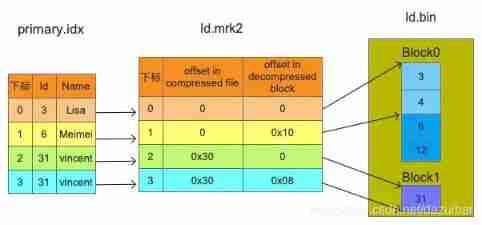
We can see from the picture , The data marker and index interval are aligned , All in accordance with index_granularity Granularity interval of , In this way, you can directly find the corresponding data mark by simply indexing the subscript number . And in order to connect with the data ,.bin Files and data mark files are one-to-one correspondence , Per one [Column].bin There's a file [Column].mrk Data mark file corresponding to it , Used to record data in .bin Offset information in the file .

A row of marked data is represented by a tuple , The tuple contains the offset information of two integer values , It respectively indicates that in this data range ：

1\. Corresponding .bin In the compressed file , The starting offset of the compressed data block
2\. Decompress the data block , Starting offset of uncompressed data

A row of marked data is represented by a tuple , The tuple contains the offset information of two integer values . They respectively represent within this data interval , In the corresponding ．bin In the compressed file , The starting offset of the compressed data block ; And decompressing the data compression block , The starting offset of its uncompressed data . The figure shows ．mrk Schematic diagram of marked data in the file .

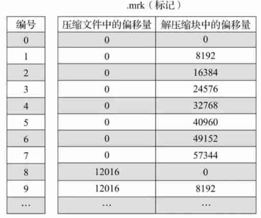
Each row of tag data represents a fragment of data （ Default 8192 That's ok ） stay ．bin Read location information in compressed file . Tag data is different from primary index data , It does not reside in memory , But use LRU（ Recently at least use ） Cache policy speeds up its access .

compressed data

The amount of data is relatively small , The size of each column of data is not very large , Therefore, each column can be stored with only one compressed data block . If there is more data , A compressed data block cannot be stored , Then it will correspond to multiple compressed data blocks .

Column1  Compressed data block 0
Column2  Compressed data block 0
Column3  Compressed data block 0
......
ColumnN  Compressed data block 0

Column1  Compressed data block 1
Column2  Compressed data block 1
Column3  Compressed data block 1
......
ColumnN  Compressed data block 1

Column1  Compressed data block 2
Column2  Compressed data block 2
Column3  Compressed data block 2
......
ColumnN  Compressed data block 2

Column1  Compressed data block 3
Column2  Compressed data block 3
Column3  Compressed data block 3
......

Compressed data block

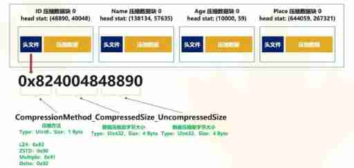
A compressed data block consists of header information and compressed data . Header information is fixed 9 Bit byte means , Specific reasons 1 individual UInt8（1 byte ） Integer sum 2 individual UInt32（4 byte ） Integer composition , Each represents the type of compression algorithm used 、 The data size after compression and the data size before compression .

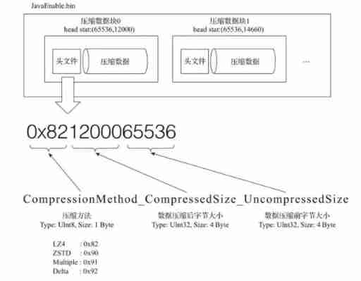
As can be seen from the figure ,.bin A compressed file is composed of multiple compressed data blocks , The header information of each compressed data block is based on CompressionMethod_CompressedSize_UncompressedSize Formula generated . adopt ClickHouse Provided clickhouse-compressor Tools , Be able to query a ．bin Statistics of compressed data in the file .

One .bin File is made up of 1 Composed of multiple compressed data blocks , The size of each compressed block is 64KB～1MB Between . Between multiple compressed data blocks , End to end in writing order , Closely arranged .

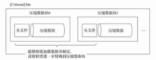
stay .bin There are at least two purposes for introducing compressed data blocks into the file ：

firstly , Although the compressed data can effectively reduce the data size , Reduce storage space and accelerate data transmission efficiency , But the compression and decompression of data , It will also bring additional performance loss . Therefore, it is necessary to control the size of compressed data , In order to find a balance between performance loss and compression ratio .

second , When specifically reading a column of data （.bin file ）, First, you need to load the compressed data into memory and decompress , In this way, subsequent data processing can be carried out . By compressing data blocks , You can read the whole... Without reading .bin In the case of files, reduce the reading granularity to the compressed data block level , So as to further reduce the range of data reading .

Partition index minmax_[Column].idx

partition.dat and minmax_[Column].idx： If the partition key is used , For example, above PARTITION BY toYYYYMM(JoinTime), Will generate additional partition.dat And minmax_JoinTime.idx Index file , They are stored in binary format .

partition.dat Used to save the final value generated by the partition expression under the current partition , and minmax_[Column].idx It is responsible for recording the minimum and maximum values of the original data corresponding to the partition fields under the current partition .

data Partitioning

ClickHouse Support PARTITION BY Clause , When creating a table, you can specify data partition operation according to any legal expression , Such as through toYYYYMM() Partition data by month 、toMonday() Partition the data by the day of the week 、 Yes Enum Type of column directly for each value as a partition, etc .

data Partition stay ClickHouse There are two main applications in ：

stay partition key On the partition cutting , Query only the necessary data . agile partition expression Set up , So that it can be based on SQL Pattern Set up the partition , Maximum fit business characteristics .
Yes partition Conduct TTL management , Obsolete data partitions .

data TTL

In the analysis scenario , The value of data decreases over time , Most businesses only keep data from recent months for cost reasons ,ClickHouse adopt TTL Provides data lifecycle management capabilities .

ClickHouse Support several different granularity of TTL：

1） Column level TTL： When part of the data in a column has expired , Will be replaced with the default value ; When the full column of data has expired , The column will be deleted .

2） Row level TTL： When a line has expired , The line will be deleted directly .

3） Division level TTL： When the partition expires , The partition will be deleted directly .

Data writing process

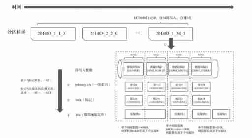
Partition Directory 、 Indexes 、 The schematic diagram of the generation process of marked and compressed data is as follows ：

Generate partition Directory

The first step in data writing is to generate a partition Directory , With the writing of each batch of data , Will generate a new partition Directory . At a later point , Directories belonging to the same partition are merged together according to rules .

Build index

according to index_granularity Index granularity , Will be generated separately primary.idx primary key （ If a secondary index is declared , It also creates secondary index files ）.

Generate tags and data compression files

according to index_granularity Index granularity , Generate .mrk Data markers and .bin Compressed data file .

ClickHouse Data query process

Overview of data query

The essence of data query , It can be seen as a process of continuously reducing the data range . In the best case ,MergeTree First, you can use the partition index in turn 、 Primary and secondary indexes , Reduce the data scanning range to a minimum . Then mark with the help of data , Reduce the range of data to be decompressed and calculated to a minimum .

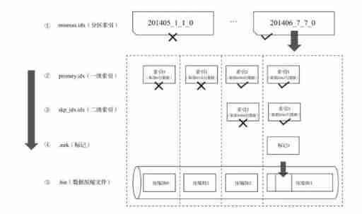
If a query statement does not specify any WHERE Conditions , Or specified WHERE Conditions , But the condition does not match any index （ Partition index 、 Primary and secondary indexes ）, that MergeTree You can't reduce the data range in advance .

During subsequent data query , It will scan all partition directories , And the maximum range of index segments in the directory . Although the data range cannot be reduced , however MergeTree Can still be marked with data , Read multiple compressed data blocks simultaneously in the form of multithreading , To improve performance .

Query process of index

Index query is actually the intersection judgment of two numerical intervals .

among , An interval is a condition interval converted from query conditions based on primary key ; And the other section is just mentioned and MarkRange The corresponding numerical interval . The figure below briefly describes Id Field indexing process .

The whole index query process can be divided into three steps

1. Generate query condition interval ： Convert query criteria into condition interval . Even the value of a single query condition , It will also be converted into interval form .

WHERE ID = 'A000' 
= ['A000', 'A000']

WHERE ID > 'A000'
= ('A000', '+inf')

WHERE ID < 'A000' 
= ('-inf', 'A000')

WHERE ID LIKE 'A000%' 
= ['A000', 'A001')

2. Recursive intersection judgment ： In the form of recursion , In turn MarkRange Make intersection judgment between the numerical interval and the conditional interval . From the largest interval [A000 , +inf) Start .

(1) If there is no intersection , Then the whole segment is optimized directly by pruning algorithm MarkRange
(2) If there is an intersection , And MarkRange The step size is larger than N, Then this interval is further divided into N Sub interval , And repeat this rule ,(3) Continue to make recursive intersection judgment （N from merge_tree_coarse_index_granularity Appoint , The default value is 8）, If there is an intersection , And MarkRange It can't be broken down , Record MarkRange And back to .

3. Merge MarkRange Section ： Will finally match MarkRange Get together , Merge their scope .

summary

Partition 、 Indexes 、 Summary of the collaborative work of marking and compressing data

Partition 、 Indexes 、 Marking and compressing data , Is similar to the MergeTree A set of combined fists , The power of using the right words is infinite . Then after introducing their respective characteristics in turn , Now put them together to summarize .

Write process

The first step in data writing is to generate a partition Directory , With the writing of each batch of data , Will generate a new partition Directory . At a later point , Partition directories belonging to the same partition will be merged . Then according to index_granularity Index granularity , Will be generated separately primary.idx First level index （ If a secondary index is declared , It also creates secondary index files ）、 Compressed data file for each column field （.bin） And data mark file （.mrk）, If the amount of data is small , It is data.bin and data.mrk file .

The following diagram shows MergeTree Table when writing data , Its partition Directory 、 Indexes 、 Generation of marked and compressed data .

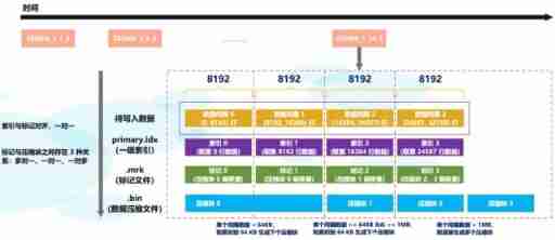
From the partition Directory 202006_1_34_3 Can know , The partition data is divided into 34 Batch write , During this period 3 The merger . During data writing , basis index_granularity Granularity , An index is generated for the data of each interval in turn 、 Mark and compress data blocks . Where the index and the marking interval are aligned , The marking and compression blocks are based on the size of the interval , Will generate many to one 、 one-on-one 、 One to many relationship .

The query process

The essence of data query can be seen as a process of constantly reducing the scope of data , In the best case ,MergeTree First, partition index 、 The primary and secondary indexes minimize the data scanning range . Then mark with the help of data , Reduce the range of data to be decompressed and calculated to a minimum . The following is an example , The figure shows that in the optimal case , After layers of filtration , Finally, the process of obtaining the minimum data range .

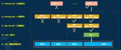
If a query statement does not specify any WHERE Conditions , Or it specifies WHERE Conditions 、 But there is no match to any index （ Partition index 、 First level index 、 Secondary indexes ）, that MergeTree You can't reduce the data range in advance . During subsequent data query , It will scan all partition directories , And the maximum range of index segments in the directory . However, although the data range cannot be reduced , but MergeTree Can still be marked with data , Read multiple compressed data blocks simultaneously in the form of multithreading , To improve performance .

The correspondence between the data mark and the compressed data block

Due to the division of compressed data blocks , With an interval （index_granularity） The size of the data in the , The volume of each compressed data block is strictly controlled at 64KB ~ 1MB Between , And an interval （index_granularity） The data of , Only one row of data markers will be generated . Then, according to the actual byte size of data in an interval , There are three different relationships between data tags and compressed data blocks ：

1） For one more

Multiple data tags correspond to a compressed data block , When an interval （index_granularity） The uncompressed size of the internal data is less than 64KB when , This correspondence will appear .

2） one-on-one

A data tag corresponds to a compressed data block , When an interval （index_granularity） The uncompressed size of internal data is greater than or equal to 64KB And is less than or equal to 1MB when , This correspondence will appear .

3） One to many

One data tag corresponds to multiple compressed data blocks , When an interval （index_granularity） The uncompressed size of the internal data is greater than 1MB when , This correspondence will appear .

That's all MergeTree How it works , First of all, we understand MergeTree Basic properties and physical storage structure ; next , Data partitioning is introduced in turn 、 First level index 、 Secondary indexes 、 Important features of data storage and data marking ; In the end, the paper summarizes the research results MergeTree The above features work together . Mastered MergeTree That is, I have mastered the essence of the merge tree series table engine , because MergeTree It is also a table engine . Later we will introduce MergeTree How to use other common table engines in the family , And what are their characteristics 、 How to use it .