当前位置:网站首页>E-commerce data analysis -- salary prediction (linear regression)
E-commerce data analysis -- salary prediction (linear regression)
2022-07-06 12:00:00 【Want to be a kite】
E-commerce data analysis – Salary forecast ( Linear regression )
Data analysis process :
- Clear purpose
- get data
- Data exploration and preprocessing
- Analyze the data
- Come to the conclusion
- Verification conclusion
- Result presentation
Linear regression : Linear regression is to use regression analysis in mathematical statistics , A statistical analysis method to determine the quantitative relationship between two or more variables , It's widely used . It is expressed in the form of y = w’x+e,e The mean value of error is 0 Is a normal distribution . In regression analysis , Include only one independent variable and one dependent variable , And the relationship between them can be approximately expressed by a straight line , This kind of regression analysis is called univariate linear regression analysis . If the regression analysis includes two or more independent variables , And the relationship between dependent variable and independent variable is linear , It is called multiple linear regression analysis .( Commonly used in demand forecasting 、 Sales forecast 、 Ranking forecast )
Univariate linear regression equation : y = b + a X y=b+aX y=b+aX
b Is the intercept ,a Is the slope of the regression line
Multiple linear regression equation : y = b 0 + b 1 X 1 + b 2 X 2 + . . . + b n X n y=b0+b1X1+b2X2+...+bnXn y=b0+b1X1+b2X2+...+bnXn
b 0 by often Count term , b 1 , b 2 , b 3 , b n by y Yes Should be And X 1 , X 2 , X 3.. X n Of partial return return system Count . b0 Constant term ,b1,b2,b3,bn by y Corresponding to X1,X2,X3..Xn Partial regression coefficient of . b0 by often Count term ,b1,b2,b3,bn by y Yes Should be And X1,X2,X3..Xn Of partial return return system Count .
skearn library - Linear regression (LinearRegression)
Specific parameter interpretation and call method :
from sklearn.linear_model import LinearRegression
LinearRegression(fit_intercept=True,normalize=False.copy_x=True,n_jobs=1)
Parameter meaning :
1、fit_intercept: Boolean value , Specify whether to calculate the intercept in linear regression , namely b value . If False, Then don't count b value .
2、normalize: Boolean value . If False, Then the training samples will be normalized .
3、copy_x: Boolean value . If True, Will copy a copy of training data ,
4、n_jobs: An integer . Specified when tasks are parallel CPU Number . If the value is -1 Then use all available CPU.
attribute :
1、coef_: The weight vector
2、intercept_: intercept b value
Method :
1、fit(X,y): Training models
2、predict(X): Use the model of training number to predict , And return the predicted value .
3、score(X,y): Return the score of prediction performance . The formula is :score=(1-u/v)
among u=((y_ture-y_pred)**2).sum(),v=((y_true-y_ture.mean())**2).sum()
score The maximum is 1, But it may be negative ( The prediction effect is too poor ).score The bigger it is , The better the prediction performance .
Salary prediction case realization
Univariate linear regression ( Working years and salary ), The data is shown in the figure .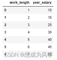
# Call the library necessary for data analysis
import numpy as np
import pandas as pd
import matplotlib.pyplot as plt
from sklearn import linear_model  # Linear model
# Import data
single_variable = pd.read_csv(r"E:\ Data analysis \ingle_variable.csv")
print(single_variable) # View the data
print(single_variable.shape)
print(single_variable.isnull().any())  # Whether there are missing values

# Prepare the data
length = len(single_variable['work_length'])
X = np.array(single_variable['work_length']).reshape([length,1])
Y = np.array(single_variable['year_salary'])
# Plot observation data
# Draw a scatter plot ,X,Y, Set the color , Mark parameters such as point style and transparency
plt.scatter(X,Y,60,color='blue',marker='o',linewidth=3,alpha=0.8)
# add to x Axis title
plt.xlabel('work years')
# add to y Axis title
plt.ylabel('year salary')
# Add chart title
plt.title('work years and year salary')
# Set the background grid line color , style , Size and transparency
plt.grid(color='#95a5a6',linestyle='--', linewidth=1,axis='both',alpha=0.4)
# Show chart
plt.show()

# Call the linear regression model
linear=linear_model.LinearRegression()
linear.fit(X,Y)
# Check intercept and coefficient
print(linear.coef_ )
print(linear.intercept_)
# Check the fitting effect score
print(linear.score(X,Y))

# New data forecast
x_new = np.array(8).reshape(1, -1)
y_pred =linear.predict(x_new)
print(y_pred)
# Finally it is concluded that  y = ax+b
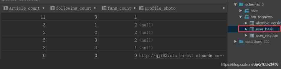
Multiple linear regression ( Years of service 、 place 、 educational level 、 Grade and salary ), The data is shown in the figure .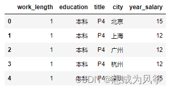
# Call the library necessary for data analysis
import numpy as np
import pandas as pd
import matplotlib.pyplot as plt
from sklearn import linear_model  # Linear model
# Import data
many_variable = pd.read_csv(r"E:\ Data analysis \many_variable.csv")
print(many_variable) # View the data
print(many_variable.shape)
print(many_variable.isnull().any())  # Whether there are missing values
# Data processing
many_variable['education']=many_variable['education'].replace([' Undergraduate ',' Graduate student '],
                    [1,2])
many_variable['city']=many_variable['city'].replace([' Beijing ',' Shanghai ',' Guangzhou ',' Hangzhou ',' Shenzhen '],
                    [1,2,3,4,5])
many_variable['title']=many_variable['title'].replace(['P4','P5','P6','P7'],
                    [1,2,3,4])
# View the data
print(many_variable)
# Prepare the data
x = np.array(many_variable[['work_length','education','title','city']])
y = np.array(many_variable['year_salary'])
# Sharding data sets ( Training set and test set )
from sklearn.model_selection import train_test_split
X_train,X_test,y_train,y_test = train_test_split(x,y,test_size=0.4,random_state=1)
# Call the linear regression model
linear2 = linear_model.LinearRegression()
linear2.fit(X_train,y_train)
# Check intercept and coefficient
print(linear2.coef_ )
print(linear2.intercept_)
# Check the fitting effect score
print(linear2.score(X,Y))

# New data forecast
y_pred =list(linear2.predict(X_test))
print(y_pred)
# Finally it is concluded that  y=1.35+1.1*work_length+5.19*education+5.92*title+0.09*city
边栏推荐
猜你喜欢

高通&MTK&麒麟 手機平臺USB3.0方案對比
RT-Thread 线程的时间片轮询调度

ToggleButton实现一个开关灯的效果
![[Flink] Flink learning](/img/2e/ff53e0795456e301f61da908c013af.png)
[Flink] Flink learning
A possible cause and solution of "stuck" main thread of RT thread
Variable star user module
Connexion sans mot de passe du noeud distribué
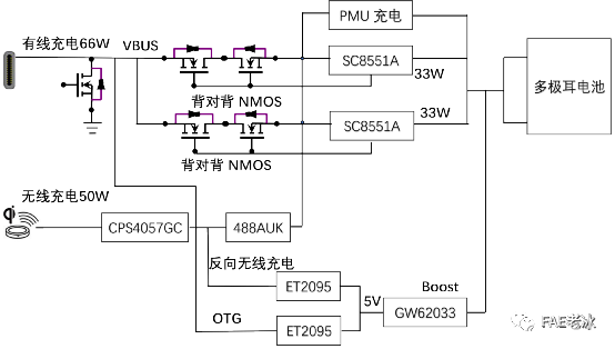
Analysis of charging architecture of glory magic 3pro
Redis面试题

5G工作原理详解(解释&图解)
随机推荐
Detailed explanation of express framework
Word typesetting (subtotal)
树莓派 轻触开关 按键使用
arduino JSON数据信息解析
Kaggle competition two Sigma connect: rental listing inquiries
Keyword inline (inline function) usage analysis [C language]
機器學習--線性回歸(sklearn)
STM32型号与Contex m对应关系
STM32 how to locate the code segment that causes hard fault
优先级反转与死锁
Word排版(小計)
列表的使用
Analysis of charging architecture of glory magic 3pro
Detailed explanation of nodejs
List and set
Comparison of solutions of Qualcomm & MTK & Kirin mobile platform USB3.0
PyTorch四种常用优化器测试
Missing value filling in data analysis (focus on multiple interpolation method, miseforest)
2020 WANGDING cup_ Rosefinch formation_ Web_ nmap
MySQL主从复制的原理以及实现