当前位置:网站首页>[classical control theory] summary of automatic control experiment
[classical control theory] summary of automatic control experiment
2022-07-05 23:21:00 【robinbird_】
※ Automatic control system script writing
1、 Variable
sym, syms Symbolic variables
sym a;
syms a b;
f = str2sym('a+ b^2');
2、 Basic operation
Derivation
dfa = diff(f function ,a For which variable ( partial ) guide );Accumulated faintness
intb = int(f function ,b Which variable to integrate ,b1,b2 Section );Laplace transform
%t You still have to define it in advance ,s Finding Laplace transform will bring
ft = exp(2*t);
L1 = laplace(ft);
Inverse Laplace transform
ftt = ilaplace(L1);
3、 Control system model
Polynomial form ( Transfer function model )
The coefficients are stored continuously in an array , An array of numerators and denominators , Pass from high to low
num = [1 2 3];  % The coefficient corresponding to the molecule
den  = [4 5 6 7]; % The coefficient corresponding to the denominator
gs = tf(num,den);
![[ Failed to transfer the external chain picture , The origin station may have anti-theft chain mechanism , It is suggested to save the pictures and upload them directly (img-doVagqrR-1657012369280)(C:\Users\robinbird\AppData\Roaming\Typora\typora-user-images\image-20220420210012659.png)]](/img/b8/1fb921cc61d3d7fa78a648738b252b.png)
![[ Failed to transfer the external chain picture , The origin station may have anti-theft chain mechanism , It is suggested to save the pictures and upload them directly (img-KrNrLKHm-1657012369284)(C:\Users\robinbird\AppData\Roaming\Typora\typora-user-images\image-20220420210717309.png)]](/img/01/eb90e5c3f6fdc64f721be991df9019.png)
Zero pole model
Two arrays are required , ditto , Add one more k gain
z = [1 2 3]';  % zero , Pay attention to add transpose
p = [4 5 6 7]; % pole
k = 9;
gs2 = zpk(z,p,k);
Interconversion
[num,den] = zp2tf(z,p,k);
% Zero pole transfer function
Other expressions
molecular / The denominator expression has zpk type , But need tf When the format , Use conv( It's polynomial multiplication ) Unified conversion to polynomial type , for example
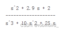
num = [1 2.9 2];
den = conv([1 0],[1 10 25]);
gs = tf(num,den);    % The root locus diagram should be drawn later
![[ Failed to transfer the external chain picture , The origin station may have anti-theft chain mechanism , It is suggested to save the pictures and upload them directly (img-joecKule-1657012369287)(C:\Users\robinbird\AppData\Roaming\Typora\typora-user-images\image-20220420211133977.png)]](/img/24/ee7194792ce5515dc8333c9ed095f2.png)
4、 Connection of models
Series connection — series
[num3,den3] = series(num,den,num2,den2);parallel connection — parallel
[num3,den3] = parallel(num,den,num2,den2);feedback — feedback
[num3,den3] = feedback(numg,deng,numh,denh,sign);
% First give G(s) Transmission characteristics of , Give again H(s) Transmission characteristics of , Last sign Is the default -1( Negative feedback ), It can be changed +1( The positive feedback )
Unit feedback — cloop
[num3,den3] = cloop(numg,deng,sign);
% Less than above H(s)
5、 Typical input function
Unit step function — step
t = [0:0.1:100];
num = 1;
den = [1 0.4 1];
step(num, den, t);
%t The main thing is to explain how long to draw t Of ct Images ,num,den Directly transfer the characteristic array of the closed-loop transfer function
Unit pulse function — impulse
t = [0:0.1:100];
num = 1;
den = [1 0.4 1];
impulse(num, den, t);
%t The main thing is to explain how long to draw t Of ct Images ,num,den Directly transfer the characteristic array of the closed-loop transfer function
Custom input — lsim
t = 0:0.1:10;

%u Contain with t The expression of , such as
u = t;
% perhaps

lsim(num,den,u,t);
lsim(z,p,k,u,t);
% It is still the beginning to give the characteristics of the closed-loop transfer function of the system , The above two forms are acceptable ,u It's input r(t), Contain with t Expression of integer ,t Is time

% for example , This is used for frequency characteristic test , Input a sine function to the system
t = [0:0.001:10];
rt = 1* sin(15 * t);
lsim(nums,dens,rt,t);
Be careful : After using all the above functions , If you use its return value , It defaults to direct single window drawing ; If you use a variable to store the return value ( It is the result of the system output , It's a one-dimensional array ), Then it can be used to draw multiple graphs
6、3 A system characteristic image
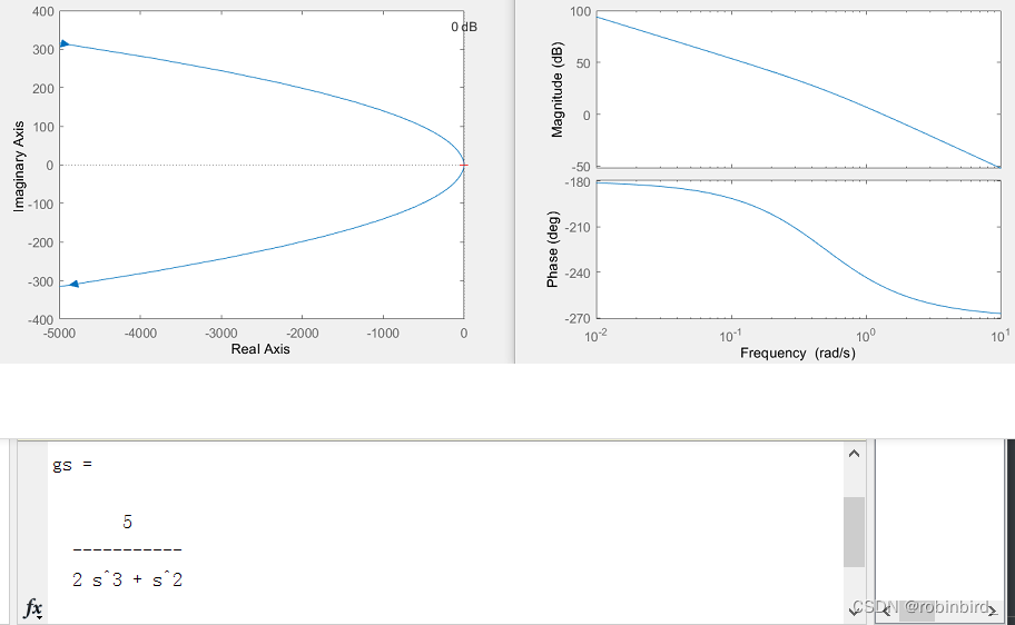
Root locus drawing
gs = tf(num,den);
rlocus(gs);  % What is given is the complete function expression , And here the first expression of the open-loop transmittal ( Without root track gain K*)
Nyquist
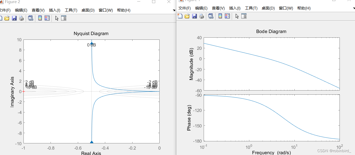
matlab The painting contains w from 0 To -∞ Track of , Completely symmetrical with the positive part , Never mind
nyquist(gs); % Pass reference pass Open loop transmittal expressionbode chart
bode(gs); % Same as before , Generally, it draws an open-loop logarithmic amplitude frequency diagram , Then give the expression of open loopfor example , Left root locus , Right bode chart
7、matlab Drawing method
Basic drawing settings
grid;  % Adding grid
xlabel(" Title name ");  % Set the name of the abscissa
ylabel(" ditto ");  % Vertical axis name
title("abb");   % The name of the drawn image
Multigraph drawing
(1) Draw a picture in one window , Be careful ,grid and legend Such special requirements do not apply to all windows , Every figure Add it separately if necessary
figure;
%code, Draw a picture

figure;
%code, Draw another picture , And so on

% give an example , First draw a bode chart , Draw another Nyquist diagram
figure;
z = [-0.2];
p = [0 -0.1 -4];
k = 16;
[num,den] = zp2tf([],[0 -4*sqrt(2)],k);
tf_gs = tf(num,den);
bode(tf_gs);

figure;
nyquist(tf_gs);
grid; %attention
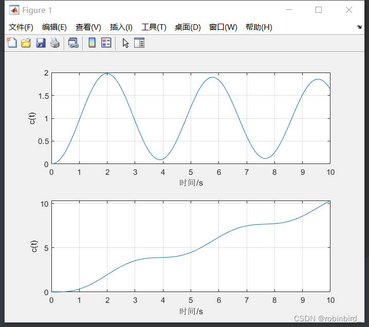
(2) Multiple graphs are drawn in one window
First of all, we need not let matlab Draw the response directly , Just use variables to receive the return value
t = 0:0.1:10; y_step = step(numfi,denfi,t); % Receive return value u = t; y_ramp = lsim(numfi,denfi,u,t); % Receive return value Then use a format similar to the previous one ,subplot Refer to this article for the parameters of :http://t.csdn.cn/pXIZ5
subplot(x1,y1,z1);
plot(t1,c1);
axis normal;

subplot(x2,y2,z2);
plot(t2,c2);
axis normal;

% give an example , Continue with the previous content
subplot(2,1,1);
plot(t,y_step);
xlabel(" Time /s");
ylabel("c(t)");
grid;
axis normal

subplot(2,1,2);
plot(t,y_ramp);
xlabel(" Time /s");
ylabel("c(t)");
axis normal
grid;
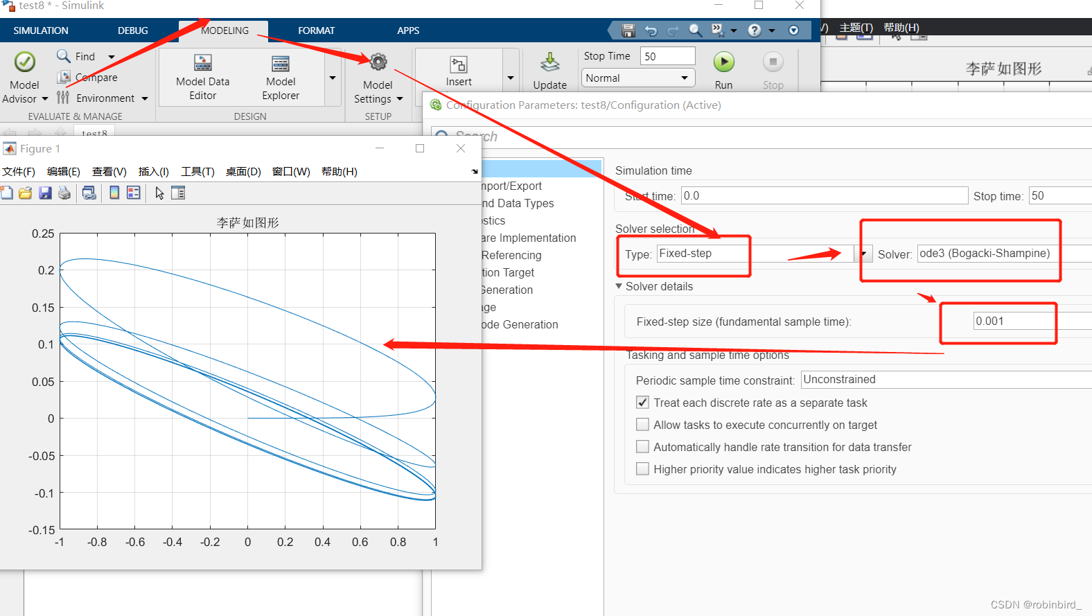
※simulink Plug in emulation
![[ Failed to transfer the external chain picture , The origin station may have anti-theft chain mechanism , It is suggested to save the pictures and upload them directly (img-WYEGSDxt-1657012369295)(C:\Users\robinbird\AppData\Roaming\Typora\typora-user-images\image-20220421104137653.png)]](/img/e5/8b609ccabbd25ebe5fbada29686760.png)
Name of common component library
And here is , Directly check the corresponding... In the component library name Search and you'll get
gain K gain
Transfer function
Polynomial type transfer fcn:
Zero pole model Zero-Pole
Oscilloscope scope
Ramp signal ramp
Step signal step
Sine signal sine wave
Sum up sum
Dead zone module dead zone
Limiting module saturation
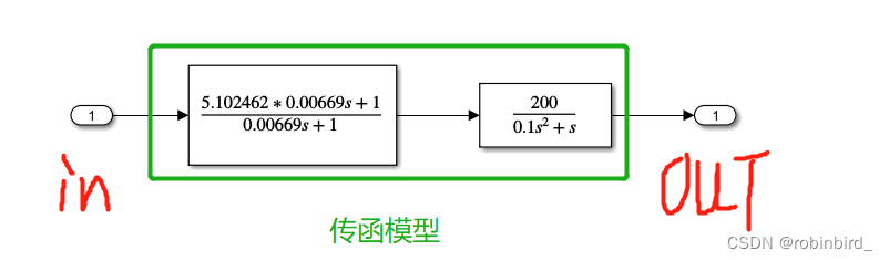
Analysis of system characteristic diagram of transfer function
First use of in and out modular , Build the following model
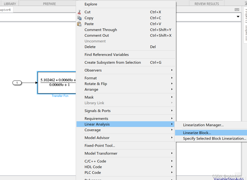
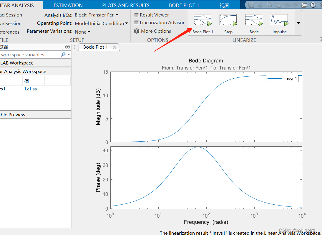
For a transmittal module , Right click , find Linearize block
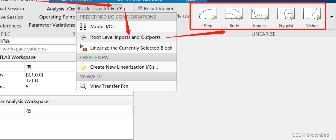
Select the source of input and output as shown in the following figure , Then click the system characteristic curve you want to obtain , You can draw directly
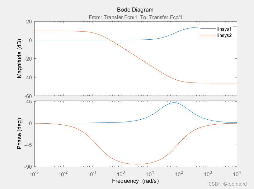
If you want to draw multiple curves on the same graph ( It is mostly used for system calibration ), Just after the first drawing ,( I'm right simulink After simply modifying the parameter value of the model ), Then click the current plot The button , There are two pictures , Stack in this way
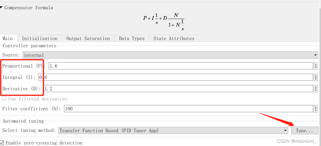
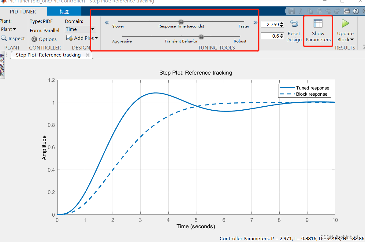
PID modular PID controller
Corresponding modification PID Three parameters are sufficient
You can also use PID tunner Instantly adjust rapidity and volatility , See the picture below
![[ Failed to transfer the external chain picture , The origin station may have anti-theft chain mechanism , It is suggested to save the pictures and upload them directly (img-22Wx11XX-1657012369297)(C:\Users\robinbird\AppData\Roaming\Typora\typora-user-images\image-20220705111245340.png)]](/img/30/5e82f63df8860ba6ab997ac7111120.png)
![[ Failed to transfer the external chain picture , The origin station may have anti-theft chain mechanism , It is suggested to save the pictures and upload them directly (img-juj7D7RC-1657012369299)(C:\Users\robinbird\AppData\Roaming\Typora\typora-user-images\image-20220421100000555.png)]](/img/73/e040fd977aec3081b9d23a8e6dfaae.png)
![[ Failed to transfer the external chain picture , The origin station may have anti-theft chain mechanism , It is suggested to save the pictures and upload them directly (img-ZF0zAQEi-1657012369301)(C:\Users\robinbird\AppData\Roaming\Typora\typora-user-images\image-20220705115014808.png)]](/img/ec/a8a894eb418c8ddbdc45f146784d73.png)
※ Scripts and simulink Dream linkage
take simulink Simulation data is used .m Script processing
Directly use the transfer function model , Through one more simout To transmit the data is
Several setting modes
structure with time
This is Time And corresponding Output
plot(out.so.time, out.so.signals.values);
%out It should be added so to simout The name of life , This can be customized , Because a .slx There can be many songs simout modular
structure
Only Output
yt = out.so.signals.values;array
Only Output , Return... As an array
plot(out.so);timeseries
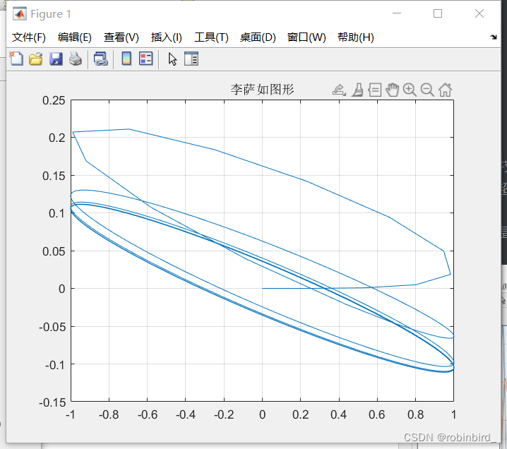
plot(out.so.Time,out.so.Data);use .m Draw Lissajou figure / Time domain response curve
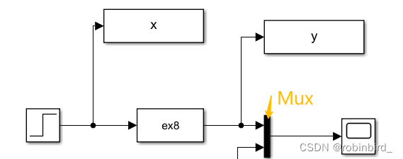
Here we directly use the code of the eighth experiment of automatic control
figure;
plot(x.signals.values,y.signals.values);
title(" Lissajous figure ");
grid;

figure;
plot(x.time,x.signals.values);
hold on;
plot(y.time,y.signals.values);
legend(" Input "," Output ");
title(" Time domain curve ");
grid;
It can be used x( Corresponding to the input of the system ), and y( Corresponding to the output of the system ) Direct use matlab fitting
Be careful : First the x,y The data type of is set to 2-D array, It's a two-dimensional array , Then follow the steps in the following article Data import :
http://t.csdn.cn/NrfDU
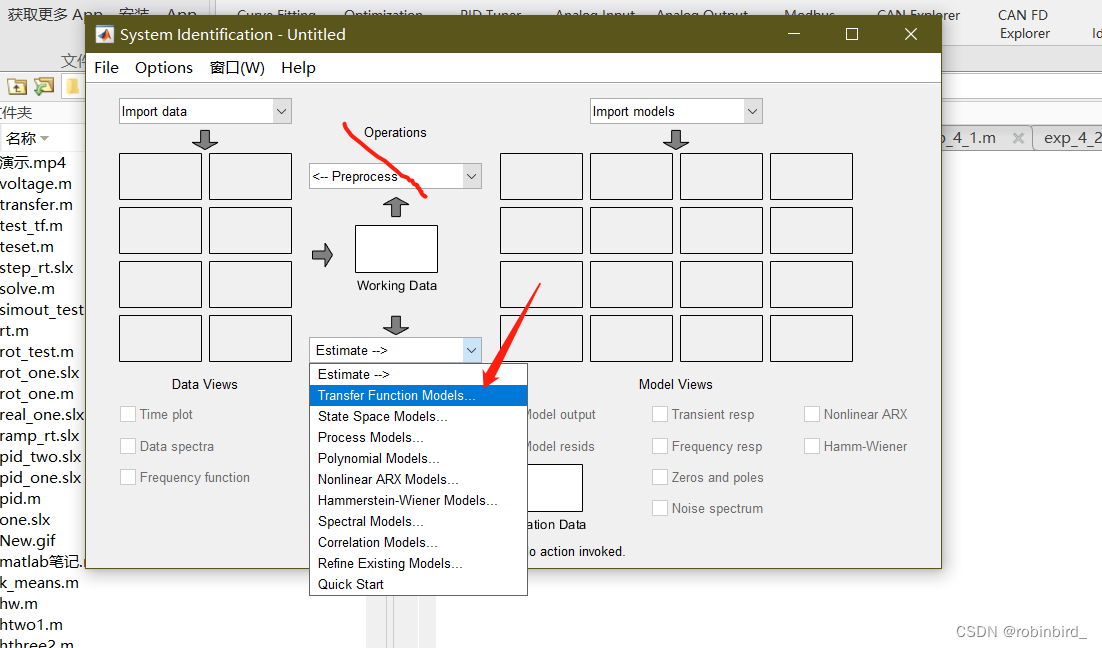
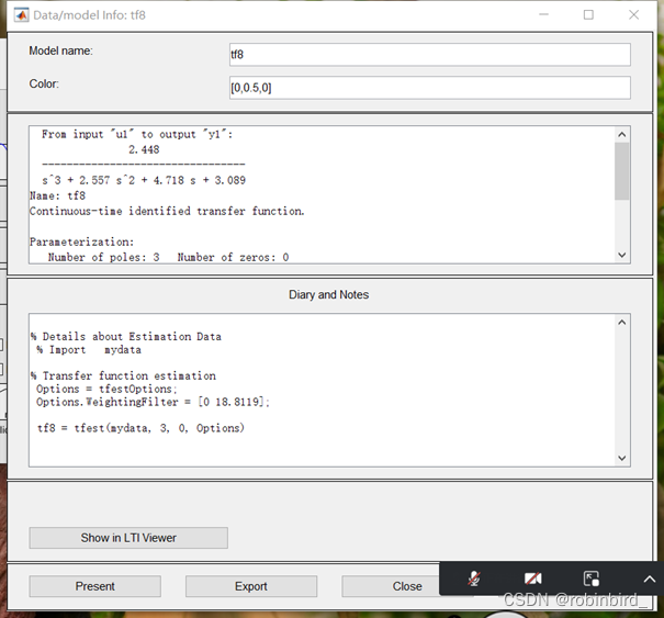
Next, analyze the link :operations Personally, I don't think it's necessary , The analysis method is the transmittal mode , You need to give the number of zeros and poles ,matlab Direct fitting according to the number of zeros and poles
Take the screenshot of your eighth experiment as an example , No zero point was selected at that time ,3 A pole
![[ Failed to transfer the external chain picture , The origin station may have anti-theft chain mechanism , It is suggested to save the pictures and upload them directly (img-N2SWPYb2-1657012369310)(C:\Users\robinbird\AppData\Roaming\Typora\typora-user-images\image-20220508110156814.png)]](/img/d3/adb265592247e13514e5e9841572e8.png)
![[ Failed to transfer the external chain picture , The origin station may have anti-theft chain mechanism , It is suggested to save the pictures and upload them directly (img-ySVKe33P-1657012369310)(C:\Users\robinbird\AppData\Roaming\Typora\typora-user-images\image-20220508110214336.png)]](/img/f4/56d245c43d21542cafd052b861faf2.png)
![[ Failed to transfer the external chain picture , The origin station may have anti-theft chain mechanism , It is suggested to save the pictures and upload them directly (img-WLfDF5oo-1657012369312)(C:\Users\robinbird\AppData\Roaming\Typora\typora-user-images\image-20220508110510079.png)]](/img/59/ef16fdd82bfb339fcca55b8ff13632.png)
※ The principle of automatic control makes up the leak ~~( A vegetable dog didn't understand until he finished the exam )~~
Mainly with The higher-order system uses the dominant pole reduction method and Frequency test of , Combined with the specific experimental content of automatic control, briefly explain
1、 Order reduction of dominant poles of higher-order systems
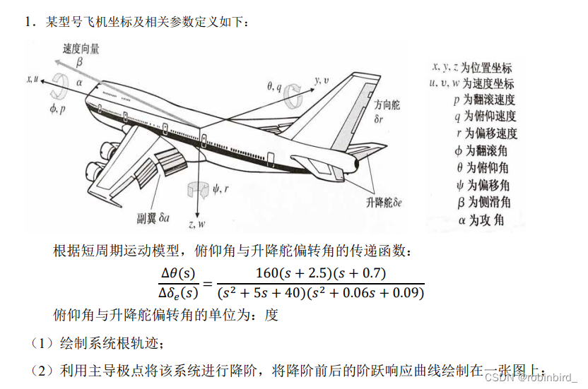
subject ( The first question is ignore ):
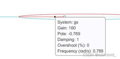
Personal understanding : The given transfer function is the open-loop transfer function of this system , And the corresponding root locus gain is 160, If you want to draw, you will get no 160 The transmittal of is passed as a parameter to rlocus Just draw ;
And for order reduction , You need to get in K*=160 All the roots of , Actually use matlab Find the root locus diagram drawn in the diagram 4 It's better to go directly to Casio 991 Solve the equation fragrant , Get more accurate results directly , See tutorial
fx-991CN X equation ( Group ) Use of solving function - Dianzhuo Yuanya Jiliang's article - You know https://zhuanlan.zhihu.com/p/28795401
Theoretical knowledge supplement : First film a wave of explanation from the giant of Harbin Industry :https://www.bilibili.com/video/BV1cK4y1U7jR?share_source=copy_web
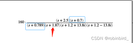
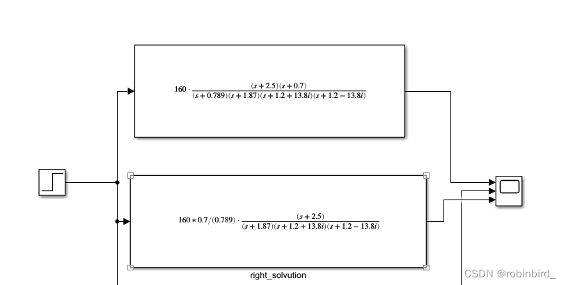
For the reduction of higher-order systems , It is necessary to ensure the stability of the system before and after order reduction Closed loop gain unchanged , So the best way is to get the closed-loop transmittal of the system , Written as closed-loop zero pole form , Then analyze the position of closed-loop zero pole , There are a pair of very close zeros and poles ( Dipole , In the blue box ), Can be removed , remainder The real part of the pole does not 2-3 Times more , Therefore, none of them can be omitted
result : according to K The unchanging principle , Whoever gets rid of it will leave the corresponding constant term , Finally, the step response curve is obtained

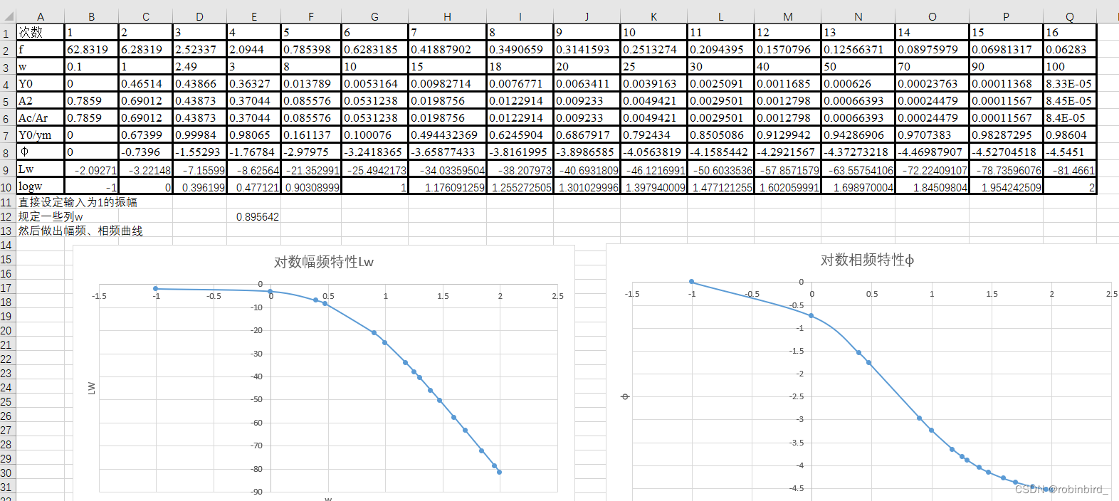
2、 Frequency characteristic test
subject :
Add :
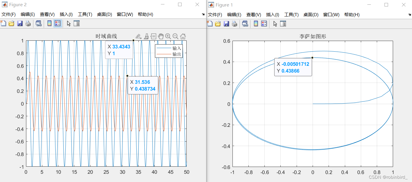
(1) The solution of phase and amplitude is as follows , So just need to be in Lissajou image (x For input ,y For export ) Found in Image and x=0 The intersection of the axes , Find in the step response curve Peak value of input / output image Put it in a table , Just draw a picture
R ( t ) = A 0 ∗ s i n ( w t ) C ( t ) = A 1 ∗ s i n ( w t + φ ) A ( w ) = A 1 / A 0 φ ( w ) = a c r s i n ( C ( 0 ) / A 1 ) R(t) = A_{0}*sin(wt)\\ C(t) = A_{1}*sin(wt+φ)\\ A(w) = A1/A0\\ φ(w) = acrsin(C(0)/A1) R(t)=A0∗sin(wt)C(t)=A1∗sin(wt+φ)A(w)=A1/A0φ(w)=acrsin(C(0)/A1)
(2) There are also aspects , Lissajou's image is elliptical , The inclination angle of its long axis ( And right x Included angle of shaft ) It's probably the phase difference , So we need to Pay attention to phase override 90°/180°/270° etc. , Modify the corresponding phase solution formula in timeLike this picture , It's a positive ellipse , The phase is close 90°
This is more than 90° 了
(3) But you can find that the curve above is not smooth enough , So I copied the similar model settings sent by the teacher before , The curve is instantly beautiful : stay simulink Look for this setting in the interface
(4) Next is excel processing section , Get organized w/A1/A0/C0 And use excel Function of , Using the type of scatter plot with asymptote , You can get the image of frequency characteristic test , And according to the maximum phase 、 The turning point 、 Initial phase 、 Initial amplitude, etc
(5) Although obviously 3 Order system , But the analysis method of second-order system is also ok 、、、 But this is not recommended ,
system identification Doesn't it smell good; Other ways , For example, some information can be obtained from the curve of step response to fit the functionIt's also a doubt that will be solved after the exam ( Pure is because he sprinkled money ):bode The picture is only for Transfer function The expression of , It has nothing to do with open-loop and closed-loop , It only uses this function The sinusoidal response result of A、φ, So all kinds of typical transmittal links in the book ( inertia 、 Oscillate 、 First and second order differential 、 Integral, etc. ) These results are applicable to the observation of frequency characteristics
![[ Failed to transfer the external chain picture , The origin station may have anti-theft chain mechanism , It is suggested to save the pictures and upload them directly (img-f2A0Bgbr-1657012369319)(C:\Users\robinbird\AppData\Roaming\Typora\typora-user-images\image-20220705161314080.png)]](/img/f1/4d9dc009701819f05ab6ab82dcd51b.png)
automatic control 1 End of the flower **ヽ(°▽°)ノ*, Already a self-control person
边栏推荐
- 2022 R2 mobile pressure vessel filling review simulation examination and R2 mobile pressure vessel filling examination questions
- YML configuration, binding and injection, verification, unit of bean
- grafana工具界面显示报错influxDB Error
- Go language implementation principle -- map implementation principle
- Scala concurrent programming (II) akka
- There are 14 God note taking methods. Just choose one move to improve your learning and work efficiency by 100 times!
- Spécifications techniques et lignes directrices pour la sélection des tubes TVS et ESD - Recommandation de jialichuang
- Basic knowledge of database (interview)
- Attacking technology Er - Automation
- Calculating the number of daffodils in C language
猜你喜欢
From the perspective of quantitative genetics, why do you get the bride price when you get married
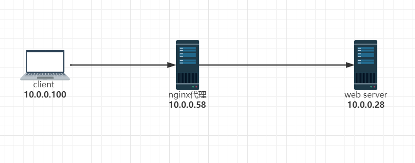
Realize reverse proxy client IP transparent transmission
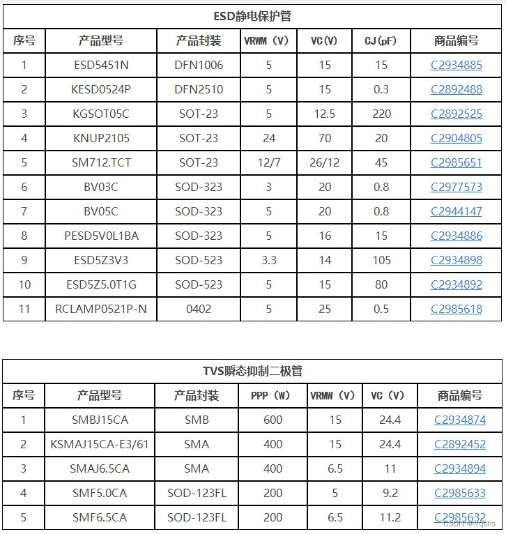
Spécifications techniques et lignes directrices pour la sélection des tubes TVS et ESD - Recommandation de jialichuang
TypeError: this. getOptions is not a function
98. 验证二叉搜索树 ●●
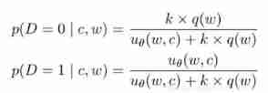
Negative sampling
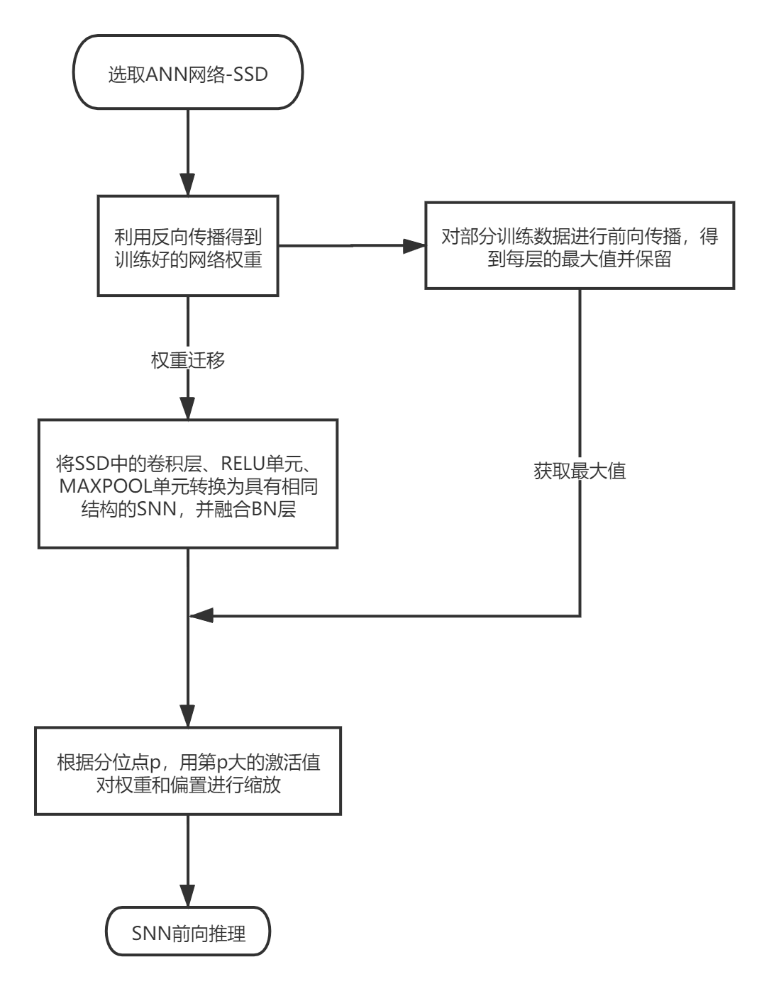
基于脉冲神经网络的物体检测
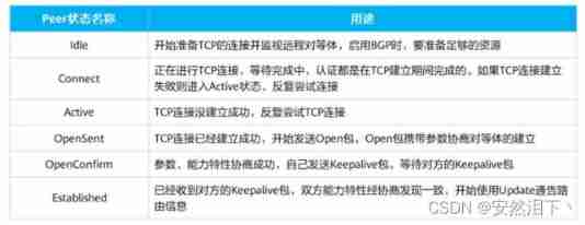
Hcip day 11 (BGP agreement)

Use of grpc interceptor
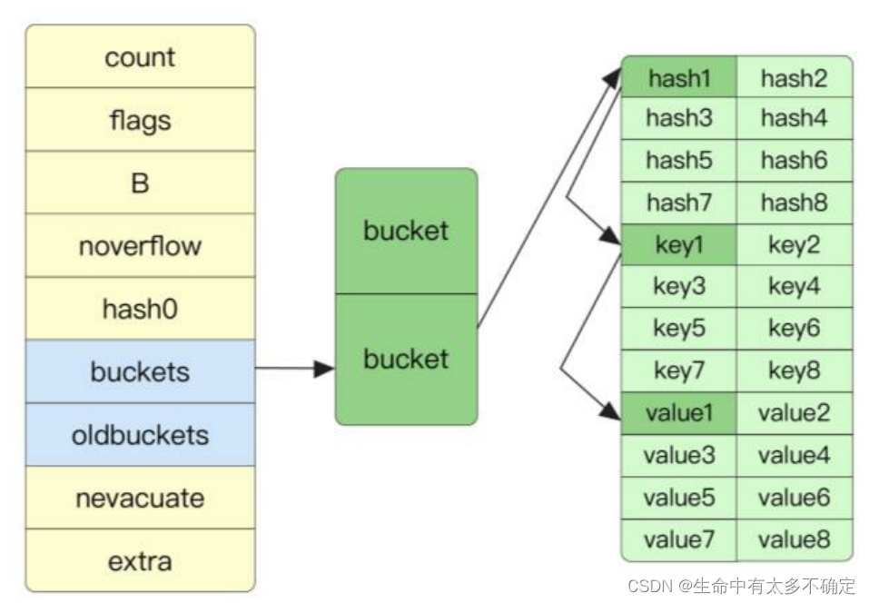
Go语言实现原理——Map实现原理
随机推荐
Mathematical formula screenshot recognition artifact mathpix unlimited use tutorial
LeetCode——Add Binary
98. 验证二叉搜索树 ●●
3: Chapter 1: understanding JVM specification 2: JVM specification, introduction;
From the perspective of quantitative genetics, why do you get the bride price when you get married
Judge whether the binary tree is a complete binary tree
Marginal probability and conditional probability
Rethinking about MySQL query optimization
Go language implementation principle -- map implementation principle
2.13 summary
Spécifications techniques et lignes directrices pour la sélection des tubes TVS et ESD - Recommandation de jialichuang
regular expression
Week 17 homework
MySQL (1) -- related concepts, SQL classification, and simple operations
Calculating the number of daffodils in C language
【经典控制理论】自控实验总结
Leetcode buys and sells stocks
Go language implementation principle -- lock implementation principle
Data type, variable declaration, global variable and i/o mapping of PLC programming basis (CoDeSys)
CJ mccullem autograph: to dear Portland