Simclr: comparative learning in NLP

Brief introduction of the paper

Thesis link ：

SimCSE: Simple Contrastive Learning of Sentence Embeddings

It's easy to do if you understand comparative learning , This article is to apply contrastive learning to the field of natural language processing . At first, learning was used in the field of images . If you understand, you can continue to read , If you don't understand it, I suggest you learn about comparative learning first . In addition, I recommend several articles written by me on comparative learning .

• The comparative study of the gods in the twilight age  

• “ The arms race ” Comparative study of the period

Unsupervised acquisition of sentence vectors ：

• Use pre trained  Bert  Get sentence vector directly , It can be  CLS  Vector of bits , It can be different  token  The average of the vectors .

• Bert-flow^[
  On the Sentence Embeddings from Pre-trained Language Models
  ], It mainly uses the flow model to correct  Bert  Vector .

• Bert-whitening^[
  Whitening Sentence Representations for Better Semantics and Faster Retrieval
  ], With pre training  Bert  Get the vectors of all sentences , Get the sentence vector matrix , Then the sentence vector matrix is transformed into a mean value through a linear transformation  0, The covariance matrix is the matrix of the unit matrix .

The main ways of supervision are :

• Sentence-Bert (SBERT)^[
  Sentence-BERT: Sentence Embeddings using Siamese BERT-Networks
  ], adopt  Bert  The twin network of gets the vector of two sentences , Conduct supervised learning ,SBERT  The structure of is shown in the figure below .

For comparative learning , The most important thing is how to construct positive and negative samples .

There are many kinds of samples for comparative learning in the image , Than SimCLR Mentioned in ： reverse 、 Partial cut 、 Local display 、 Crop flip 、 Adjust saturation 、 Adjust the color 、 Use various filters, such as maximum filter , Minimum filter 、 Sharpen the filter .

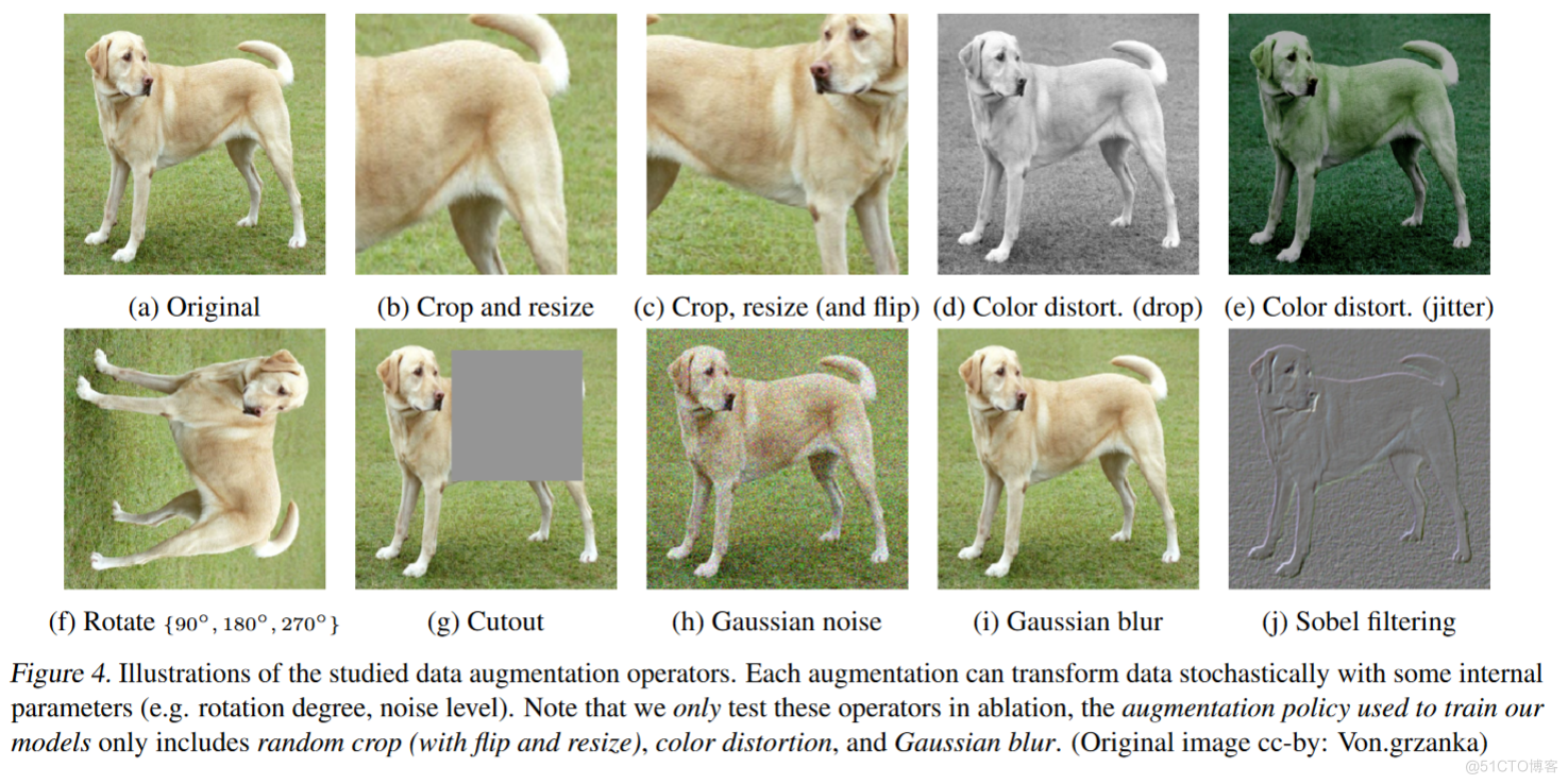
There are also many ways of data augmentation in natural language processing , But they all have a great influence on sentences . It will seriously reduce the effect of comparative learning . To solve this problem SimCSE The model proposes a method of random sampling dropout mask To construct positive samples . The model uses BERT, Every time I come out Dropout Is different . Random dropout masks The mechanism exists in the fully-connected layers and attention probabilities On , So the same input , Different results will be obtained after the model . So you only need to feed the same sentence to the model twice to get two different representations . The similar samples generated by this method are completely consistent with the semantics , It's just generated embedding It's just different , It can be considered as the smallest form of data enhancement . It is much better than other data enhancement methods .

What is? dropout

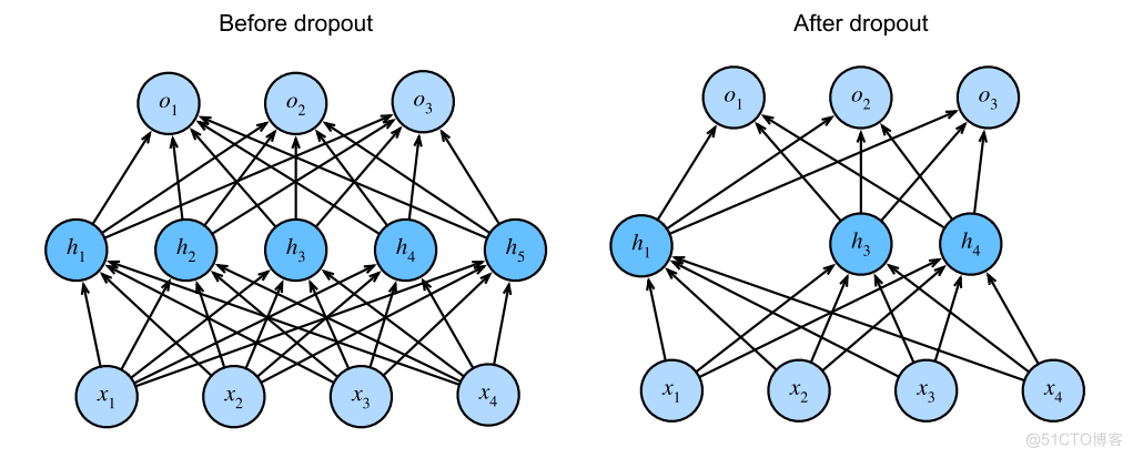
First of all, we need to understand what dropout.dropout In deep learning, it is usually used to prevent the model from over fitting .dropout By the first Hinton Group in 2014 in . Take a look at my previous post ：

Model generalization  |  Regularization  |  Weight decline  | dropout

Why is the model over fitted . Because our data set is too small compared with our model . Our model is too complex compared with our data set . Therefore, in order to prevent the model from over fitting , We can use dropout, Let the model ignore some nodes during training . Like in the picture above . This model trains different networks every time when training data , The model will not rely too much on some local features , So the generalization of the model is stronger , It reduces the probability of over fitting .

dropout Compare with other data enhancement methods

adopt dropout masks Mechanism for data enhancement to construct positive examples .

The author in STS-B Data sets . Compare dropout Differences with other data enhancement methods .

tailoring , Data enhancement methods such as deletion and replacement , The effect is not as good as dropout masks Mechanism , Even deleting a word can damage performance , The details are shown in the table below ：

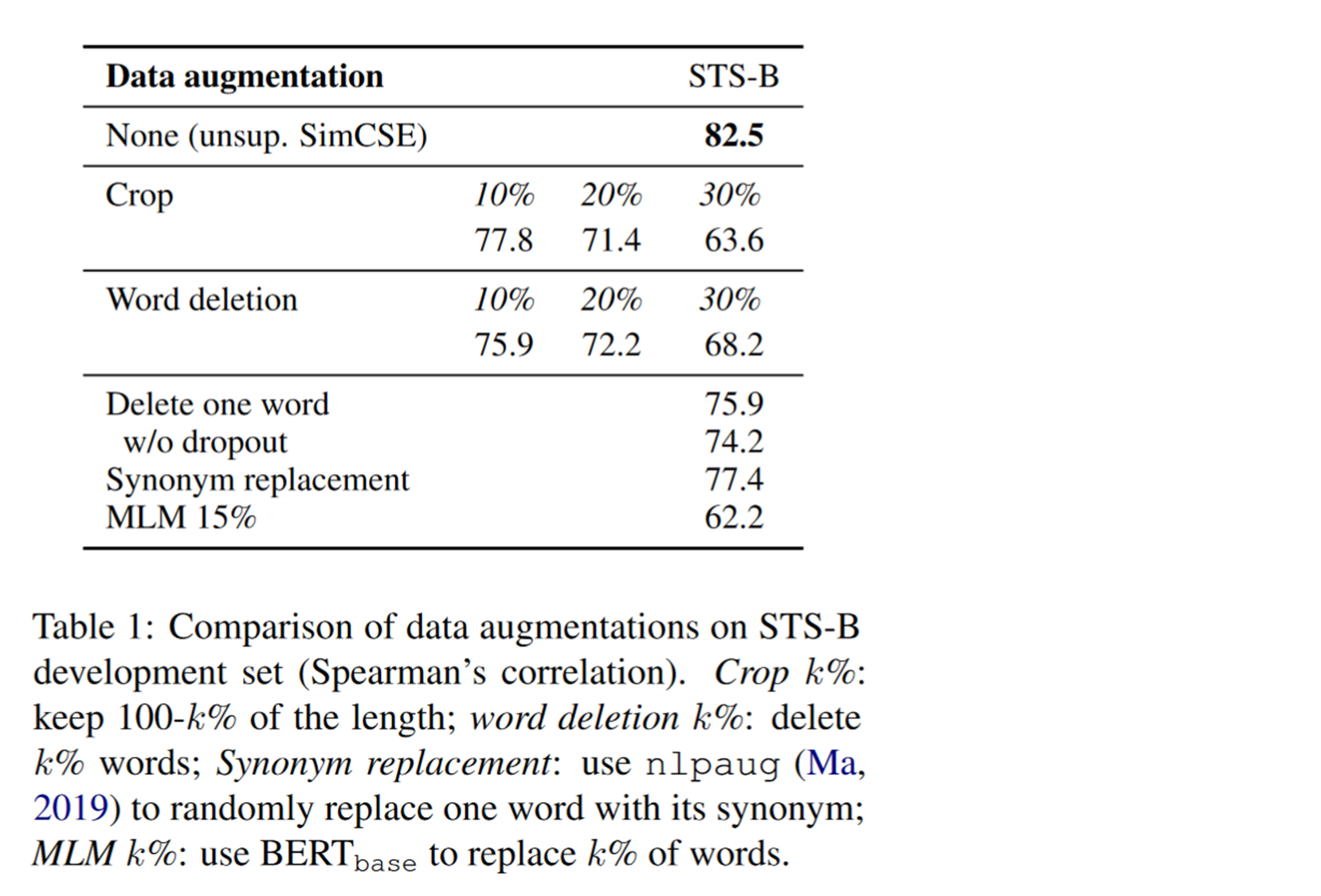
dropout The exact same sentences are used between the positive example and the original sample , Only in the process of vector representation dropout mask Somewhat different . It can be regarded as a minimum form of data expansion .

Different dropout rate

To test the model dropout rate No supervision SimCSE Influence , The author in STS-B Ablation experiments were carried out on the data set . From the table above, we can see that when dropout rate Set to 0.1 When , Model in STS-B The test set works best .

Above picture

It means to use the same... For the same sample dropout mask, That is to say, the vector obtained by encoding twice is the same , You can see that the effect is the worst in this case .

My personal feeling

Can achieve 40% The above is already very good . After all, in my eyes, it may cause the model to collapse .

I also read someone else's article reproducing this paper , The person who reappears said he tried 0.1 0.2 0.3, The effect is almost the same , Finally, I chose... In the paper 0.1. No .

Compare learning evaluation indicators

alignment  and  uniformity  They are two important attributes in comparative learning , It can be used to measure the effect of comparative learning .

• alignment  Calculate the distance between all positive sample pairs , If  alignment  The smaller it is , Then the vector of the positive sample is closer , The better the effect of comparative learning , The calculation formula is as follows ：$
  
  
  $

• uniformity  Indicates the uniformity of the distribution of all sentence vectors , Smaller means that the vector distribution is more uniform , The better the effect of comparative learning , The calculation formula is as follows ：$$\ell_{\text {uniform }} \triangleq \log \quad \mathbb{E}
  {x, y \stackrel{i . i . d .}{\sim} p
  {\text {data }}} e^{-2|f(x)-f(y)|^{2}}$$

among

Represents the data distribution . These two indicators are consistent with the goal of comparative learning ： The characteristics learned between positive examples should be similar , The semantic features of any vector should be scattered on the hypersphere as much as possible .

As for this “ hypersphere ” I think it's like InstDisc The picture on the right in the middle is the same , Map the feature representation of each sample into space .（ Personal view , If there is any mistake in understanding, please advise .）

Unsupervised

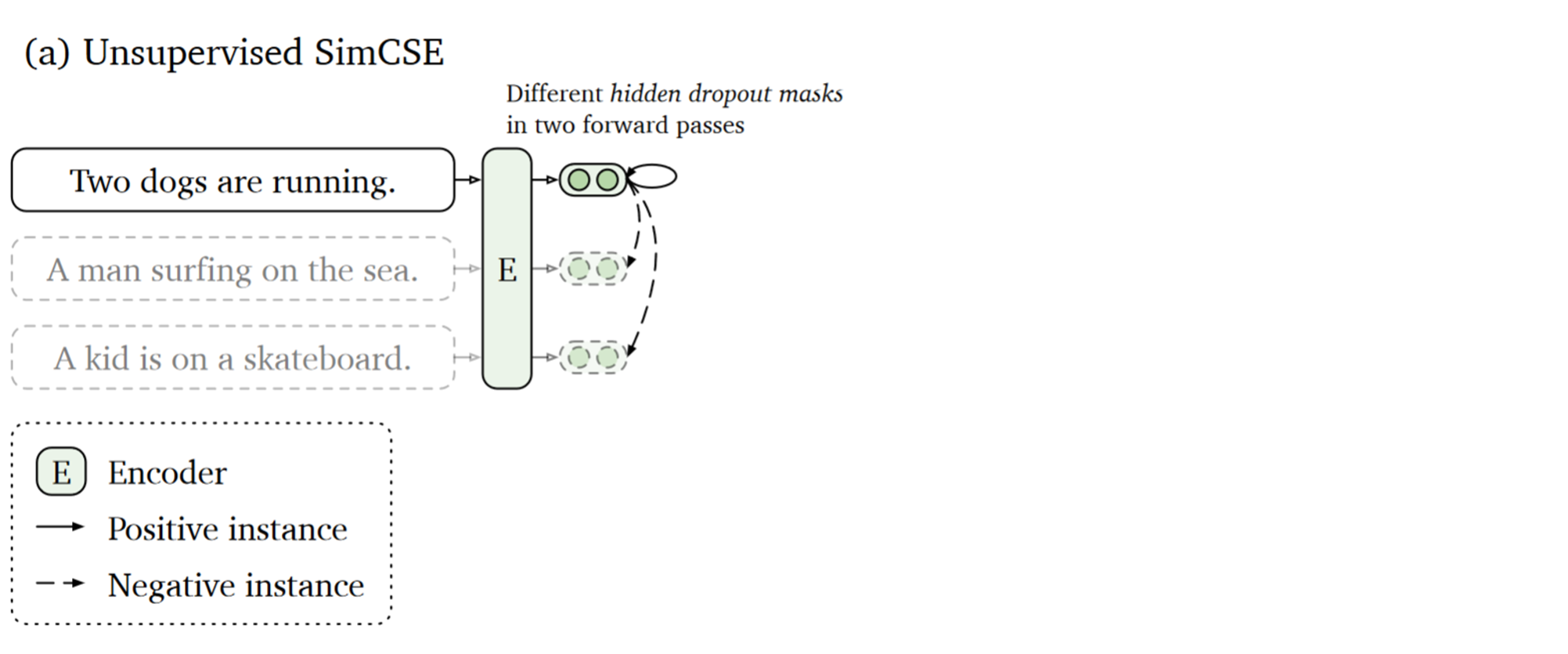
The unsupervised objective function is like this . Look at the top , The example in his figure is to send three sentences as input to the encoder , Then the encoder will get the corresponding sentence embedding. Enter twice and you will get two different embedding. A sentence and its corresponding enhanced sentence are positive samples , The rest of the sentences are taken as negative samples . The final loss function used is as follows ：$$\ell_{i}=-\log \frac{e^{\operatorname{sim}\left(\mathbf{h}

{i}^{z

{i}}, \mathbf{h}

{i}^{z

{i}^{\prime}}\right) / \tau}}{\sum_{j=1}^{N} e^{\operatorname{sim}\left(\mathbf{h}

{i}^{z

{i}}, \mathbf{h}

{j}^{z

{j}^{\prime}}\right) / \tau}}$$

Supervised

One difficulty in using supervised learning , It is to find a data set suitable for constructing positive and negative samples . The final author's choice is as follows ：

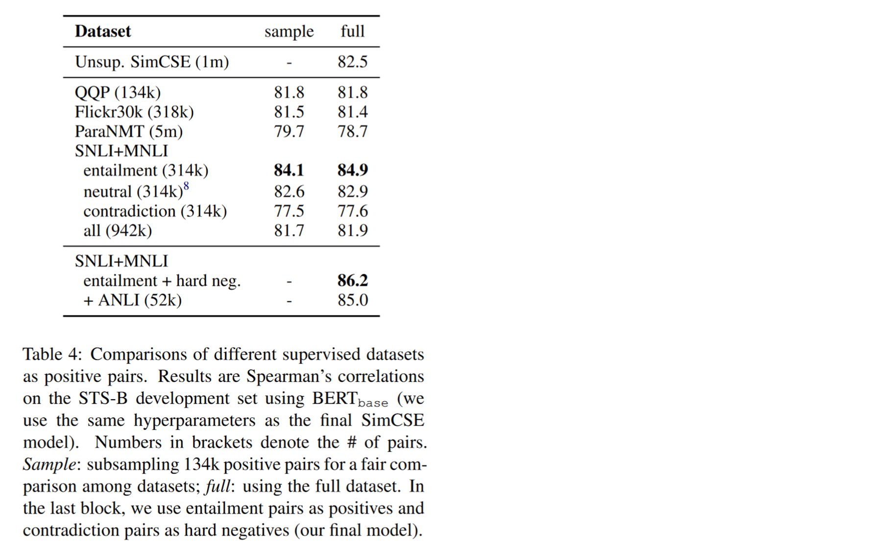
How are its positive and negative benefits constructed . With one of them NLI Data sets, for example , Enter a premise in this data set . That is, the annotator needs to manually write an absolutely correct sentence and implied sentence . A sentence that may be correct , Neutral sentences . Contradict an absolutely wrong sentence . Then this paper will expand this data set , The original （ The sentence , Contain sentences ） Change for （ The sentence , Contain sentences , Contradictory sentences ）. In this data set, the exact sample is this sentence and the sentences containing implicative relationships . There are two kinds of negative samples , It is this sentence that contains contradictory sentences and other sentences . The loss function is as follows ：

result

Yes 7 Semantic text similarity (STS) The task was tested , Will be unsupervised and supervised SimCSE And STS The most advanced sentence embedding methods in the task are compared , You can find , Unsupervised and supervised SimCSE All have achieved sota The effect of , The details are shown in the table below ：

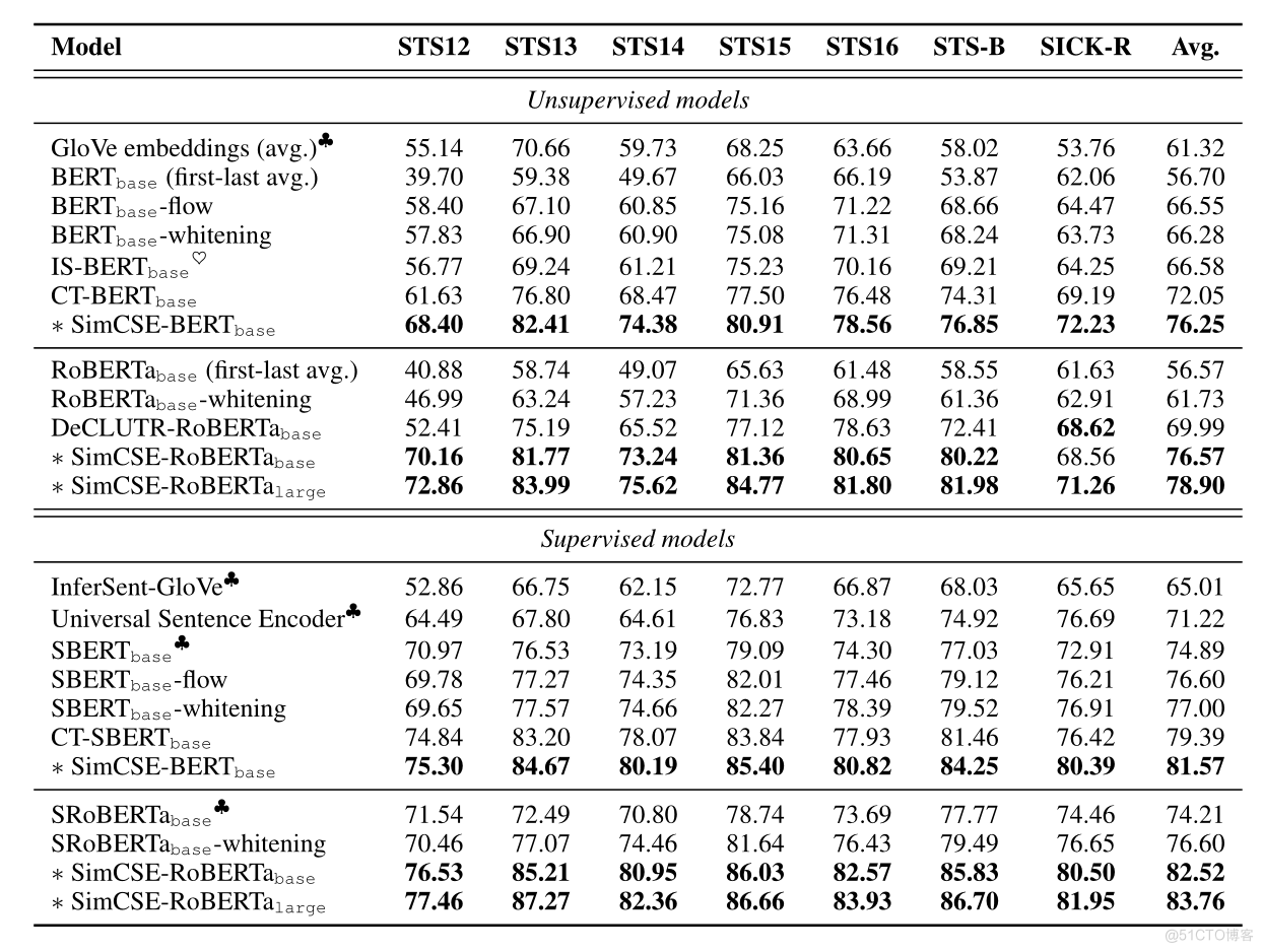
because SimCSE What we do is a task of sentence representation , That is, to get better sentences embedding, The experimental effect is shown in the figure above . The author uses BERT And based on RoBERTa Of SimCSE Respectively with Baseline Compare , Good results have been achieved .

Below is SimCSE Use different versions of BERT And its variants , The corresponding model can be directly from hugging face Get on the .

Code practice

Since its effect is so good , How to use it quickly on the computer SimCSE Well ？

Install it first ：

pip install simcse


Load the model with these two lines of code . I wrote different versions in the form above , 

SimCSE(" Fill in different versions here ")

.

from simcse import SimCSE
model = SimCSE("princeton-nlp/sup-simcse-bert-base-uncased")


Since it is used for sentence embedding Of , First, let's see how he encodes sentences ：

embeddings = model.encode("A woman is reading.")


It reacts slowly , You need to wait for it to come out . If nothing else , It should give a very long embedding code .

Let me output it and have a look , He should encode a sentence into 768 The vector of the dimension .

Calculate the ‎‎ Cosine similarity ‎：

sentences_a = ['A woman is reading.', 'A man is playing a guitar.']
sentences_b = ['He plays guitar.', 'A woman is making a photo.']
similarities = model.similarity(sentences_a, sentences_b)

similarities1 = model.similarity('A woman is reading.', 'A man is playing a guitar.')
similarities2 = model.similarity('He plays guitar.', 'A man is playing a guitar.')


In addition to calculating between sentence groups , I also put some similarities between the two sentences . The final effect is shown as follows ：

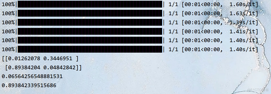
He can also construct for that group of sentences index, After construction, you enter a sentence , Find it . He will find out which sentence is more similar . And output the similarity .

sentences = ['A woman is reading.', 'A man is playing a guitar.']
model.build_index(sentences)
results = model.search("He plays guitar.")


In the last code, I have calculated the similarity between these two sentences , We can see that the result in the previous code is the same .

similarities2 = model.similarity('He plays guitar.', 'A man is playing a guitar.')

The output of is 0.8934233..... Now you check

He plays guitar.

It outputs the most similar sentences as

A man is playing a guitar.

The similarity is 0.8934233.....