当前位置:网站首页>Convolution, pooling, activation function, initialization, normalization, regularization, learning rate - Summary of deep learning foundation
Convolution, pooling, activation function, initialization, normalization, regularization, learning rate - Summary of deep learning foundation
2022-07-06 07:59:00 【The story has turned several pages】
I have the honor to read the book of big brother Yan Yousan 《 The model design of deep learning 》, Here are my reading notes , For reference only , You have to read the original work for details , Please correct the mistakes . The following three pictures are from Zhihu .
《 The model design of deep learning 》 Reading notes —— Chapter two : The foundation of deep learning
List of articles
- 《 The model design of deep learning 》 Reading notes —— Chapter two : The foundation of deep learning
- 2.1 Limitations of fully connected neural networks
- 2.2 Study the brief history of the third Renaissance in depth
- 2.3 The basis of convolutional neural network
- 2.3.1 Convolution operation
- 2.3.2 Deconvolution operation
- 2.3.3 Basic concept of convolutional neural network
- 2.3.4 The core idea of convolutional neural network
- 2.3.5 CNN Basic structure configuration of
- 2.4.1 Activation model and common activation functions
- 2.4.2 Parameter initialization method
- 2.4.3 Normalization method
- 2.4.4 Pooling
- 2.4.5 Optimization method —— Optimizer
- 2.4.6 Learning rate strategy
- 2.4.7 Regularization method
2.1 Limitations of fully connected neural networks
2.2.1 Defects of learning principles
Traditional machine learning requires artificial design of feature description operators , But people are limited after all , This limits the expression ability of the traditional fully connected neural network in principle , It can only solve relatively simple problems .
2.2.2 Structural defects of fully connected neural networks
- Huge amount of calculation
- Lack of structural information
2.2.3 High performance traditional machine learning algorithm
- Adaboost
- SVM
2.2 Study the brief history of the third Renaissance in depth
2.2.1 The Internet and big data are coming
The birth of large data sets , Many machine learning models have enough data to train models with good generalization performance .
2.2.2GPU The popularity of
1. What is? GPU
- Definition :GPU(Graphics Processing Unit) Graphics processor .
- characteristic :GPU Using a large number of computing units and ultra long pipeline , And it saves Cache.
2.GPU Architecture and software platform
GPU Programmable .
GPU Development stage : Fixed function architecture stage ⇒ \Rightarrow ⇒ Separate the rendering architecture stage ⇒ \Rightarrow ⇒ Unified rendering architecture stage
3.GPU And CPU Computational power comparison
(1)GPU The floating-point operation ability of is CPU More than ten times .
(2)GPU It has high-speed and wide independent video memory ; High floating point performance ; Strong geometric processing ability ; Suitable for processing parallel computing tasks ; Suitable for repeated calculation ; Suitable for image or video processing tasks ; It can greatly reduce the system cost .
2.2.3 The deep neural network is gorgeous
A little
2.2.4 A major breakthrough in speech recognition
A little
2.2.5 A major breakthrough in image recognition
ZFNet( deconvolution )(2013) ⇒ \Rightarrow ⇒GoogLeNet(Inception)&VGGNet(2014) ⇒ \Rightarrow ⇒ResNet(2015) ⇒ \Rightarrow ⇒ResNeXt( Grouping convolution )&DenseNet(2016) ⇒ \Rightarrow ⇒SeNet(2017)
2.2.6 A major breakthrough in natural language processing
LSTM(2014) ⇒ \Rightarrow ⇒ Attention mechanism (2014) ⇒ \Rightarrow ⇒Transformer(2017) ⇒ \Rightarrow ⇒ELMO(2017) ⇒ \Rightarrow ⇒GPT(2018) ⇒ \Rightarrow ⇒GPT2.0(2019) ⇒ \Rightarrow ⇒XLNet(2019)
2.3 The basis of convolutional neural network
2.3.1 Convolution operation
1. Mathematical convolution :
among ( x ∗ w ) ( t ) (x*w)(t) (x∗w)(t) be called x x x and w w w Convolution of
Continuous definition : ( x ∗ w ) ( t ) = ∫ − ∞ + ∞ f ( τ ) g ( t − τ ) d τ (x*w)(t)=\int_{-\infty}^{+\infty}f(\tau)g(t-\tau)d\tau (x∗w)(t)=∫−∞+∞f(τ)g(t−τ)dτ
The definition of discreteness : ( x ∗ w ) ( t ) = ∑ − ∞ + ∞ f ( τ ) g ( t − τ ) (x*w)(t)=\sum_{-\infty}^{+\infty}f(\tau)g(t-\tau) (x∗w)(t)=∑−∞+∞f(τ)g(t−τ)
2. Convolution of two-dimensional graphics :
( x ∗ w ) ( i , j ) = ∑ m ∑ n x ( m , n ) w ( i − m , j − n ) (x*w)(i,j)=\sum_m\sum_n x(m,n)w(i-m,j-n) (x∗w)(i,j)=m∑n∑x(m,n)w(i−m,j−n)
among x x x Indicates input w w w Convolution kernel .
To put it bluntly , Convolution is sliding on the image , Take a region equal in size to the convolution kernel , Multiply pixel by pixel and add .
I add : There are also three modes in convolution :
1.full mode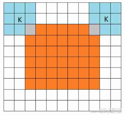
full The pattern means , from filter and image Just started convolution , The white part is filled with 0.filter The range of motion is shown in the figure .
2.same mode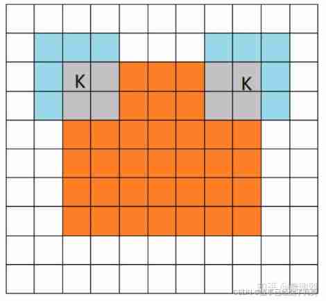
When filter Center of (K) And image When the edges and corners coincide , Start convolution , so filter The range of motion is larger than full The pattern is a little smaller . Be careful : there same There is another meaning , Output after convolution feature map The size remains the same ( Relative to the input picture ). Of course ,same Mode does not mean that the input and output dimensions are the same , It also has something to do with the step size of the convolution kernel .same Patterns are also the most common patterns , Because this mode can keep the size of the feature graph unchanged in the process of forward propagation , The parameter adjuster does not need to accurately calculate its size change ( Because the size hasn't changed at all ).
3.valid mode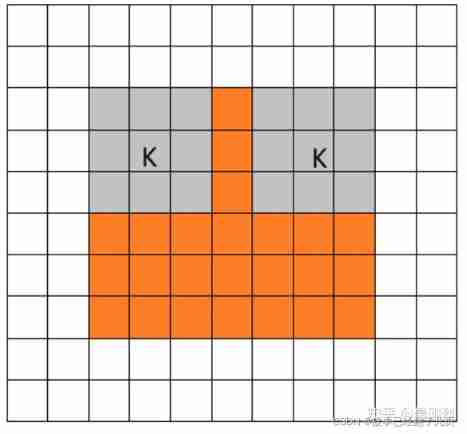
When filter All in image When it's inside , Do convolution , so filter The moving range of the is same Smaller .
2.3.2 Deconvolution operation
Convolution usually causes resolution reduction , Deconvolution is just the opposite .
actually , There is no such operation as deconvolution , Currently in DeepLearning There are mainly two ways to realize deconvolution —— Interpolation and transpose convolution
1. Interpolation method
Four points are known Q 11 = ( x 1 , y 1 ) , Q 12 = ( x 1 , y 2 ) , Q 21 = ( x 2 , y 1 ) , Q 22 = ( x 2 , y 2 ) Q_{11}=(x_1,y_1),Q_{12}=(x_1,y_2),Q_{21}=(x_2,y_1),Q_{22}=(x_2,y_2) Q11=(x1,y1),Q12=(x1,y2),Q21=(x2,y1),Q22=(x2,y2)
Yes x x x Linear difference in direction :
f ( x , y 1 ) ≈ x 2 − x x 2 − x 1 f ( Q 11 ) + x − x 1 x 2 − x 1 f ( Q 21 ) f(x,y_1)\approx \dfrac{x_2-x}{x_2-x_1} f(Q_{11}) + \dfrac{x-x_1}{x_2-x_1}f(Q_{21}) f(x,y1)≈x2−x1x2−xf(Q11)+x2−x1x−x1f(Q21)
f ( x , y 2 ) ≈ x 2 − x x 2 − x 1 f ( Q 12 ) + x − x 1 x 2 − x 1 f ( Q 22 ) f(x,y_2)\approx \dfrac{x_2-x}{x_2-x_1} f(Q_{12}) + \dfrac{x-x_1}{x_2-x_1}f(Q_{22}) f(x,y2)≈x2−x1x2−xf(Q12)+x2−x1x−x1f(Q22)
Then on y y y Linear difference in direction :
f ( x , y ) ≈ y 2 − y y 2 − y 1 f ( x , y 1 ) + y − y 1 y 2 − y 1 f ( x , y 2 ) f(x,y)\approx \dfrac{y_2-y}{y_2-y_1} f(x,y_1) + \dfrac{y-y_1}{y_2-y_1}f(x,y_2) f(x,y)≈y2−y1y2−yf(x,y1)+y2−y1y−y1f(x,y2)
First pair y The direction is again right x The result of directional interpolation is the same .
2. Transposition convolution ( deconvolution )
In fact, it is also a convolution operation , Use the same code as convolution .
In practice , First calculate Up sampling magnification ( transport Out ruler " transport Enter into ruler " \dfrac{ Output size }{ Enter dimensions } transport Enter into ruler " transport Out ruler " ). According to Step Size and Boundary supplement To transform the initial input . Then use the same method as convolution to learn parameters .
2.3.3 Basic concept of convolutional neural network
1. Feel the field
stay CNN in , It is a mapping of the input layer corresponding to an element of the output result of a certain layer , That is, the area on the input image corresponding to a point on the feature plane .
If the size of a neuron is affected by the upper layer N × N N \times N N×N The influence of neuronal regions , So the receptive field of this neuron is N × N N \times N N×N, Because it reacts N × N N \times N N×N Regional information .
2. Pooling
Realization way :
1. step Not for 1 Convolution of ;
2. Direct sampling .
The pooling layer can compress the input feature plane , Sure :
1. Make the feature plane smaller , Simplify network computing complexity ;
2. Extract the main features .
Common pooling is :
Average Pooling、Max Pooling.
2.3.4 The core idea of convolutional neural network
1. Sparse connection
Most of the neurons in the anterior and posterior layers are connected locally .
The source of thought : Physiological receptive field mechanism and Local statistical properties of images
2. Weight sharing
Weight sharing in the same feature plane .
The information learned in the local area of the image can be applied to other areas , So that the same target can extract the same features in different positions .
3. Can model image structure information
The preservation of spatial relations is CNN The basis for extracting robust features
2.3.5 CNN Basic structure configuration of
- Input layer : Contains basic operations : If you go to the mean value , Gray normalization
- Convolution layer
- Activation layer : Select and suppress features
- Pooling layer : Reduce the resolution and abstract features of the plane ; Compress network parameters and data , Reduce over fitting
- Fully connected layer
- Loss layer ; Define the loss objective function ( Such as SGD), Find the parameter value of the minimization loss function ( The input of the loss layer is the output of the network and the real label )
- Precision layer : The input is the output of the network and the real label
2.4.1 Activation model and common activation functions
1. Linear model and threshold model
2. Activation function
- Sigmoid: f ( x ) = 1 1 + e − x f(x)=\dfrac{1}{1+e^{-x}} f(x)=1+e−x1
- Tanh: f ( x ) = e x − e − x e x + e − x f(x)=\dfrac{e^{x}-e^{-x}}{e^{x}+e^{-x}} f(x)=ex+e−xex−e−x It's solved Sigmoid The output value of the function does not begin with 0 Centered problem
- ReLU
- Leaky ReLU: f ( x ) = m a x ( 0.01 x , x ) f(x)=max(0.01x,x) f(x)=max(0.01x,x), It's solved Dead ReLU problem , But it has not been completely proved to be better than ReLU
- PreLU: take Leaky ReLU Medium α \alpha α Set as a parameter that can be learned
- Maxout: y = m a x ( a k ) = m a x ( w 1 T x + b 1 , w 2 T x + b 2 , . . . , w n T x + b n ) y=max(a_k)=max(w_1^Tx+b_1,w_2^Tx+b_2,...,w_n^Tx+b_n) y=max(ak)=max(w1Tx+b1,w2Tx+b2,...,wnTx+bn) Consider adding an activation function layer to the network , It contains a parameter k, The special thing is that k Neurons , And output the maximum activation value .
have ReLU All the advantages of functions , There are no shortcomings .
Can fit any convex function .
and Dropout The combined use effect is better . - Softmax: f ( x 1 ) = e x i ∑ k = 1 K e x k f(x_1)=\dfrac{e^{x_i}}{\sum^{K}_{k=1}e^{x_k}} f(x1)=∑k=1Kexkexi As Sigmoid The generalized form of .
- Swish: f ( x ) = x ∗ S i g m o i d ( β x ) f(x)=x*Sigmoid(\beta x) f(x)=x∗Sigmoid(βx) , It is an activation function automatically searched by the network , among β \beta β Is a parameter or constant that can be learned .
3. Research direction of activation function
1. Yes ReLU Improve the negative region of the function
2. Study different activation strategies for different network layers 、 The impact of different channel use
3. Use various learning methods to explore simple combinations
at present ,ReLU Functions are still the most common .
2.4.2 Parameter initialization method
principle :
- The activation value of each layer will not be saturated
- The activation value of each layer is not 0
Ideal initialization : Make the activation value of each layer consistent with the variance of the state gradient in the propagation process
1. Initialize to 0
Not conducive to optimization
2. Generate small random numbers
Gaussian distribution can be used
The initial value of the parameter cannot be too small : Smaller parameters will cause too small gradients when propagating , For deep Networks , Will produce gradient dispersion .
The initial value of the parameter cannot be too large : Cause oscillation , Also can make Sigmoid Enter the gradient saturation zone .
3. Standard initialization
4.Xavier initialization
5.MSRA initialization
6. Use of initialization methods
- Use a trained model ( The best initialization method )
- Choose a better activation function :
MSRA Initialization method +ReLU Series collocation —— The current mainstream
2.4.3 Normalization method
Definition : Normalization is to constrain data to a fixed distribution range .
1.Normalization
- Linear contrast stretch : X = x − x m i n x − x m a x X=\dfrac{x-x_{min}}{x-x_{max}} X=x−xmaxx−xmin , among x m i n x_{min} xmin and x m a x x_{max} xmax They are the minimum and maximum gray values .
- Histogram equalization : Let one transform from random distribution to [0,1] Uniformly distributed transformation .
Transformation steps :
(1) Calculate cumulative probability distribution , c d p ( r k ) cdp(r_k) cdp(rk) Indicates that the gray scale is 0 − r k 0-r_k 0−rk The probability of pixels . c d p ( L − 1 ) = 1 cdp(L-1)=1 cdp(L−1)=1. c d p ( r k ) = ∑ i = 0 L − 1 p ( r k ) , k = 0 , 1 , 2... L − 1 cdp(r_k)=\sum^{L-1}_{i=0}p(r_k),k=0,1,2...L-1 cdp(rk)=∑i=0L−1p(rk),k=0,1,2...L−1
(2) Create a uniform distribution , Convert the cumulative probability distribution to the pixel range of the image , The transformation relation is : T ( r k ) = r o u n d ( c d p ( r k ) ∗ 255 + 0.5 ) T(r_k)=round(cdp(r_k)*255+0.5) T(rk)=round(cdp(rk)∗255+0.5), among r o u n d round round Indicates rounding operation . T ( r k ) T(r_k) T(rk) stay ( 0 , 255 ) Inside (0,255) Inside (0,255) Inside
(3) Reverse mapping , New pixel gray value after transformation y y y With the original pixel gray value x x x The transformation relation of is y = T ( x ) y=T(x) y=T(x) - Zero mean normalization : The average value of the processed data is 0, The standard deviation is 1 The standard normal distribution of . y i = x i − u δ y_i=\dfrac{x_i - u}{\delta} yi=δxi−u
2.Batch Normalization
Usually BN The layer is behind the convolution layer , Used to redistribute data .
ensp Average value of each batch : u B = 1 n ∑ i = 1 n x i u_B = \dfrac{1}{n} \sum^n_{i=1} x_i uB=n1∑i=1nxi
Variance of each batch :$\delta^2_B = \dfrac{1}{n} \sum^n_{i=1} (x_i-u_B)^2 $
Normalize each element : x i ′ = x i − u B δ B 2 + ε x^{'}_i = \dfrac{x_i-u_B}{\sqrt{\delta^2_B+\varepsilon}} xi′=δB2+εxi−uB
Scaling and shifting : y i = γ i × x i ′ + β i y_i = \gamma_i \times x^{'}_i + \beta_i yi=γi×xi′+βi, among , γ \gamma γ and β \beta β Represents the variance and offset of the input data distribution .
CNN Each characteristic dimension of ( passageway ) Between , It is conducted separately BN Calculated .
BN The benefits of :1. Reduce the dependence on the initial value 2. Faster training , You can use a higher learning rate
BN The shortcomings of : rely on Batch Size , When Batch It's worth a lot of time , The calculated mean and variance are unstable . Therefore, it is not suitable for 1.Batch A very small 2. A model with variable depth , Such as RNN
3.Batch Renormalization
BN With each Batch To replace the mean and variance of the overall training set , This requires Batch Samples must be taken evenly from all types , When Batch When the value is small, it is difficult to meet this requirement .
and Batch Renormalization And then we can solve this problem .
take BN Change the corresponding formula in :
x i ′ = x i − u B δ β . r + d x^{'}_i = \dfrac{x_i- u_B}{\delta_{\beta}}. r + d xi′=δβxi−uB.r+d
among r = δ β δ r=\dfrac{\delta_\beta}{\delta} r=δδβ, d = u β − u δ d=\dfrac{u_\beta-u}{\delta} d=δuβ−u
among u : = u + α ( u β − u ) u:=u+\alpha(u_\beta-u) u:=u+α(uβ−u), δ : = δ + α ( u β − δ ) \delta:=\delta+\alpha(u_\beta-\delta) δ:=δ+α(uβ−δ)
In practice , First use BN Train the network to a relatively stable moving average , Reuse Batch Renormalization Training .
4.BN variant
- Layer Normalization(LN): Apply to RNN Equal time series model
- Instance Normalization(IN): Suitable for image generation and style transfer
- Generalized Normalization(GN): Apply to Batch smaller
- Switchable Normalization(SN): Choose from the pool containing the normalization method , And then compare the accuracy to select the best , Finally, the best configuration is learned adaptively in the task . The specific result may be : When the batch processing is smaller ,BN The more unstable , The smaller the corresponding weight coefficient ,IN and LN The larger the weight coefficient of ; conversely BN The larger the weight coefficient of ( A bit like a random forest ).
2.4.4 Pooling
1. Based on the scheme of manually designing pooling
- Average Pooling
- Max Pooling
- Mixed Pooling: stay Average Pooling and Max Pooling Random selection in , It can provide certain regularization ability
- Stochastic Pooling: Yes feature map The elements in are randomly selected according to the size of the probability value , The probability of an element being selected is positively correlated with its value .
2. Data driven pooling scheme
Under study
3. Understanding of pooling mechanism
effect : Translation invariance is increased to a certain extent
It doesn't play a big role in the deep network , What is really useful is data enhancement .
2.4.5 Optimization method —— Optimizer
- SGD(Stochastic Gradient Descent): Only one sample is selected at a time for gradient calculation
- RMSProp
- AdaGrad
- NAG(Nesterov Accelerated Gradient)
- Adam: It's essentially a momentum term REMSProp
- Adamax: The upper limit of learning rate provides a simpler range
- Nadam: with Nesterov Of momentum terms Adam
- Newton method
- Quasi Newton method
- conjugate gradient method
2.4.6 Learning rate strategy
The more late in training , The lower the learning rate , Contribute to the stability of convergence
- Fixed: Fixed learning rate strategy
- Step: Adjust the learning rate according to the specified step . Such as : Learning rate every time 10000 After the second iteration, it is reduced to the original 0.1 times
- Multistep: Non uniform step size reduction strategy
- Exp: Index change strategy
- Inv: Another index change strategy
- Poly: Another index change strategy
- Sigmoid
2.4.7 Regularization method
1. Over fitting and under fitting
- Over fitting (Overfitting): The data set is very small or The model is too big —— resolvent : Regularization and data expansion
- Under fitting (Underfitting): Not trained enough
2. Regularization
- Regularization (Regularization): The goal is : Let experience risk and model complexity be smaller at the same time . effect : The generalization error is reduced by increasing the error of the training set .
3. Early stop
After the verification error no longer increases , Finish training early
Strategies for making full use of training data sets :1. Train all training data together for a fixed number of iterations 2. Iterative training process , Until the training error is less than the verification error of the early stop strategy setting .
4. Model integration
- Model Ensemble Methods: Combine the results of multiple models to get a better model
- dropout
5. Parameter penalty
6. Training sample expansion
- CV in : Rotate the picture 、 The zoom 、 Translation, etc
- NLP in : Synonym replacement, etc
- In speech recognition : Add random noise, etc
边栏推荐
- edge浏览器 路径获得
- esRally国内安装使用避坑指南-全网最新
- "Designer universe" APEC design +: the list of winners of the Paris Design Award in France was recently announced. The winners of "Changsha world center Damei mansion" were awarded by the national eco
- Data governance: 3 characteristics, 4 transcendence and 3 28 principles of master data
- The difference between TS Gymnastics (cross operation) and interface inheritance
- 1202 character lookup
- Asia Pacific Financial Media | "APEC industry +" Western Silicon Valley invests 2trillion yuan in Chengdu Chongqing economic circle to catch up with Shanghai | stable strategy industry fund observatio
- 好用的TCP-UDP_debug工具下载和使用
- 数据治理:误区梳理篇
- Description of octomap averagenodecolor function
猜你喜欢
It's hard to find a job when the industry is in recession
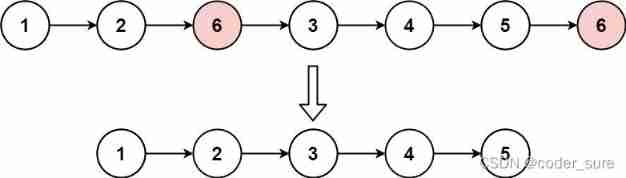
Leetcode question brushing record | 203_ Remove linked list elements

Go learning notes (3) basic types and statements (2)
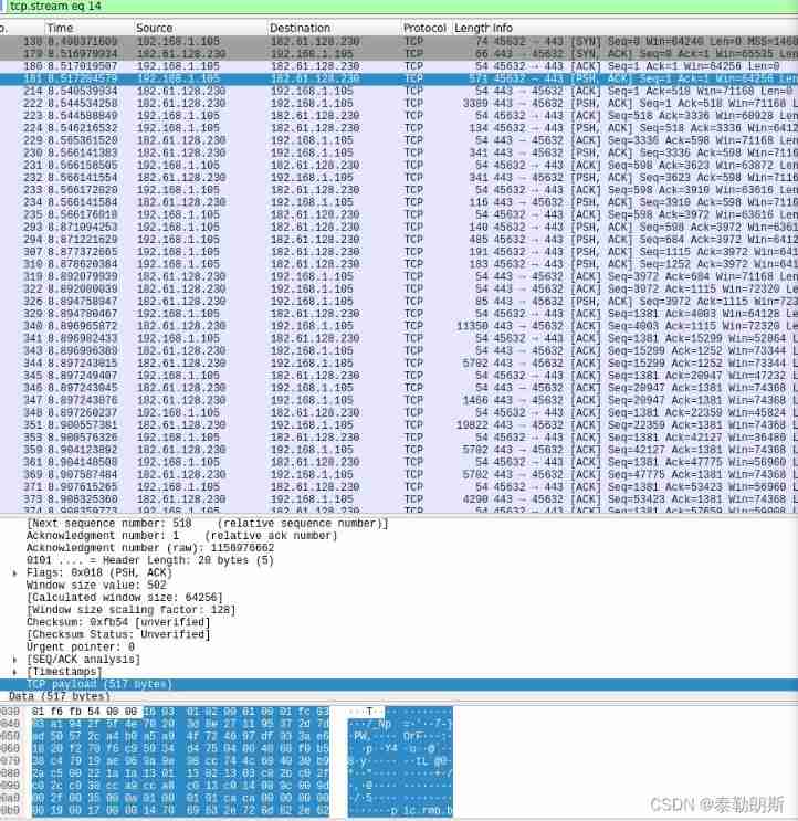
Wireshark grabs packets to understand its word TCP segment
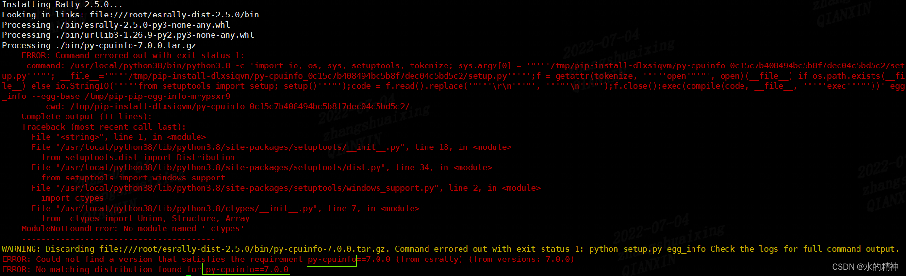
Esrally domestic installation and use pit avoidance Guide - the latest in the whole network
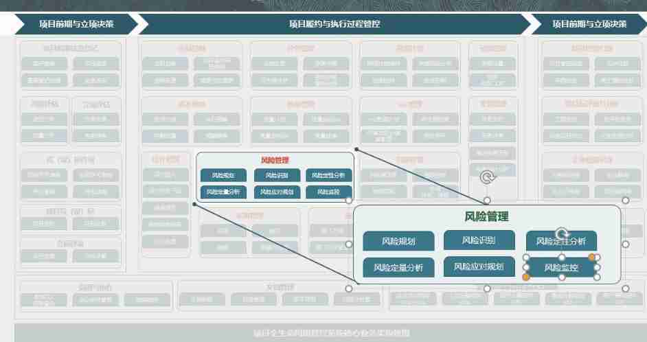
Qualitative risk analysis of Oracle project management system
Solution: intelligent site intelligent inspection scheme video monitoring system
Risk planning and identification of Oracle project management system

The ECU of 21 Audi q5l 45tfsi brushes is upgraded to master special adjustment, and the horsepower is safely and stably increased to 305 horsepower
Make learning pointer easier (3)
随机推荐
CAD ARX gets the current viewport settings
[KMP] template
Asia Pacific Financial Media | art cube of "designer universe": Guangzhou community designers achieve "great improvement" in urban quality | observation of stable strategy industry fund
It's hard to find a job when the industry is in recession
Data governance: data quality
Nft智能合约发行,盲盒,公开发售技术实战--合约篇
链表面试题(图文详解)
onie支持pice硬盘
Golang DNS write casually
Luogu p4127 [ahoi2009] similar distribution problem solution
Onie supports pice hard disk
Linked list interview questions (Graphic explanation)
C # display the list control, select the file to obtain the file path and filter the file extension, and RichTextBox displays the data
[count] [combined number] value series
WebRTC系列-H.264预估码率计算
. Net 6 learning notes: what is NET Core
[redis] Introduction to NoSQL database and redis
Helm install Minio
Generator Foundation
"Designer universe": "benefit dimension" APEC public welfare + 2022 the latest slogan and the new platform will be launched soon | Asia Pacific Financial Media