Structural theme model (I) STM package workflow

Structure theme model （ One ）stm Package workflow

Preface

On the thesis (stm: An R Package for Structural Topic Models) in stm Code workflow , The overall structure refers to the original paper , But I put forward my own ideas about the sequence of some code execution . Because time is limited , There are unresolved errors and problems （ For example, choose the appropriate number of topics 、 Draw a time trend chart ……）, The later part of the paper is not described in detail , I hope a friend can put forward effective suggestions for modification , Bloggers will give feedback at the first time . Last , Hope to use STM Friends of structural theme model are helpful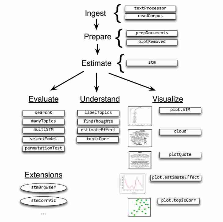

3.0 Reading data

Sample data poliblogs2008.csv For a blog post on American politics , come from CMU2008 Political blog corpus ：American Thinker, Digby, Hot Air, Michelle Malkin, Think Progress, and Talking Points Memo. Every blog forum has its own political tendencies , So every blog has metadata of writing date and political ideology .

# data <- read.csv("./poliblogs2008.csv", sep =",", quote = "", header = TRUE, fileEncoding = "UTF-8")
data <- read_excel(path = "./poliblogs2008.xlsx", sheet = "Sheet1", col_names = TRUE)

With 3.0 The starting number is to keep consistent with the original paper

3.1 Ingest: Reading and processing text data

Extract the data ： Process the raw data into STM Three pieces of content that can be analyzed （ Namely documents,vocab ,meta）, What is used is textProcessor or readCorpus These two functions .

textProcessor() The function is designed to provide a convenient and fast way to process relatively small text , In order to use the software package for analysis . It aims to quickly capture data in a simple form , For example, spreadsheets , Each of these documents is in a single cell .

#  call textProcessor Algorithm , take  data$document、data  As a parameter 
processed <- textProcessor(documents = data$documents, metadata = data)

It is mentioned in the paper that ,textProcessor() Can handle multiple languages , Variables need to be set language = "en", customstopwords = NULL,. Bloggers did not try

See ：textProcessor function - RDocumentation

3.2 Prepare: Associating text with metadata

Data preprocessing ： Transform data format , Delete low-frequency words according to the threshold , What is used is prepDocuments() and plotRemoved() Two functions

plotRemoved() Function can draw deleted under different thresholds document、words、token Number

pdf("output/stm-plot-removed.pdf")
plotRemoved(processed$documents, lower.thresh = seq(1, 200, by = 100))
dev.off()

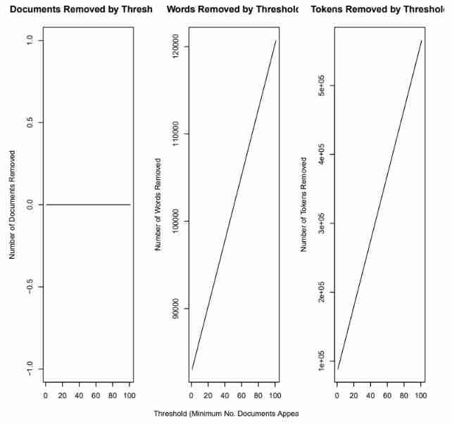
According to this pdf Results of documents （output/stm-plot-removed.pdf）, determine prepDocuments() Parameters in lower.thresh The value of , To determine the variable docs、vocab、meta

It is mentioned in the paper that if there is any change in the process ,PrepDocuments All metadata will also be re indexed / Document relationships . for example , When the document is completely deleted in the preprocessing stage because it contains low-frequency words , that PrepDocuments() The corresponding row in the metadata will also be deleted . Therefore, after reading and processing text data , It is important to check the characteristics of documents and related vocabularies to ensure that they have been preprocessed correctly .

#  Remove words with frequency lower than 15 's vocabulary 
out <- prepDocuments(documents = processed$documents, vocab = processed$vocab, meta = processed$meta, lower.thresh = 15)

docs <- out$documents
vocab <- out$vocab
meta <- out$meta

• docs：documents. A list of documents containing word indexes and their associated counts

• vocab：a vocab character vector. Contains the words associated with the word index

• meta：a metadata matrix. Contains document covariates

The following are two short articles documents： The first article contains 5 Word , Each word appears in vocab vector Of the 21、23、87、98、112 position , Except that the first word appears twice , The rest of the words appear only once . The second article contains 3 Word , The explanation is the same as above .

[[1]]
	[,1]	[,2]	[,3]	[,4]	[,5]
[1,]	21	23	87	98	112
[2,]	2	1	1	1	1
[[2]]	[,1]	[,2]	[,3]
[1,]	16	61	90
[2,]	1	1	1

3.3 Estimate: Estimating the structural topic model

STM The key innovation of is it Merge metadata into the theme modeling framework . stay STM in , Metadata can be input into the topic model in two ways ：** Theme popularity （topical prevalence）** And theme content （topical content）. Metadata covariates in topic popularity allow observed metadata to affect the frequency of topics being discussed . Covariates in topic content allow observed metadata to affect word usage within a given topic —— That is, how to discuss specific topics . The estimation of theme popularity and theme content is through stm() Functionally progressive .

Theme popularity （topical prevalence） Indicates the contribution of each topic to a document , Because different documents come from different places , Therefore, we naturally hope that the popularity of topics can change with the change of metadata .

To be specific , The paper will variable rating（ ideology ,Liberal,Conservative） As a covariate of topic popularity , Except ideology , You can also use + Add other covariates , Such as adding day” Variable （ Indicates the posting date ）

s(day) Medium s() by spline function,a fairly flexible b-spline basis

day This variable is derived from 2008 From the first day to the last day of the year , It's like panel data equally , If the carry in sequence is set to day （365 individual penal）, Will lose 300 Multiple degrees of freedom , So the introduction of spline function Solve the problem of freedom loss .

The stm package also includes a convenience functions(), which selects a fairly flexible b-spline basis. In the current example we allow for the variabledayto be estimated with a spline.

poliblogPrevFit <- stm(documents = out$documents, vocab = out$vocab, K = 20, prevalence = ~rating + s(day), max.em.its = 75, data = out$meta, init.type = "Spectral")

R The covariate of topic popularity prevalence It can be expressed as a formula containing multiple oblique variables and factorials or continuous covariates , stay spline package There are other standard conversion functions in ：log()、ns()、bs()

As the iteration goes on , If bound The change is small enough , It is considered that the model converges converge 了 .

3.4 Evaluate: Model selection and search

1. Model initialization for a fixed number of topics Create an initialization model for a specified number of topics

Because the posterior of mixed topic model is often non convex and difficult to solve , The determination of the model depends on the starting value of the parameter （ for example , Word distribution for a specific topic ）. There are two ways to implement model initialization ：

• spectral initialization.init.type="Spectral". This method is preferred
• a collapsed Gibbs sampler for LDA

poliblogPrevFit <- stm(documents = out$documents, vocab = out$vocab, K = 20, prevalence = ~rating + s(day), max.em.its = 75, data = out$meta, init.type = "Spectral")

2. Model selection for a fixed number of topics Select a model for a specified number of topics

poliblogSelect <- selectModel(out$documents, out$vocab, K = 20, prevalence = ~rating + s(day), max.em.its = 75, data = out$meta, runs = 20, seed = 8458159)

selectModel() First, build a network of running models （net）, And run all models in turn （ Less than 10 Time ）E step and M step, Abandon low likelihood Model of , Then only run high likelihood Before 20% Model of , Until it converges （convergence） Or reach the maximum number of iterations （max.em.its）

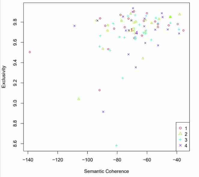
adopt plotModels() Semantic consistency of function display （semantic coherence） And exclusivity （exclusivity） Choose the right model ,semcoh and exclu The larger the model, the better

#  Draw the average score of the graph. Each model uses different legends 
plotModels(poliblogSelect, pch=c(1,2,3,4), legend.position="bottomright")
#  Choose a model 3
selectedmodel <- poliblogSelect$runout[[3]]

3. Model search across numbers of topics Determine the appropriate number of topics

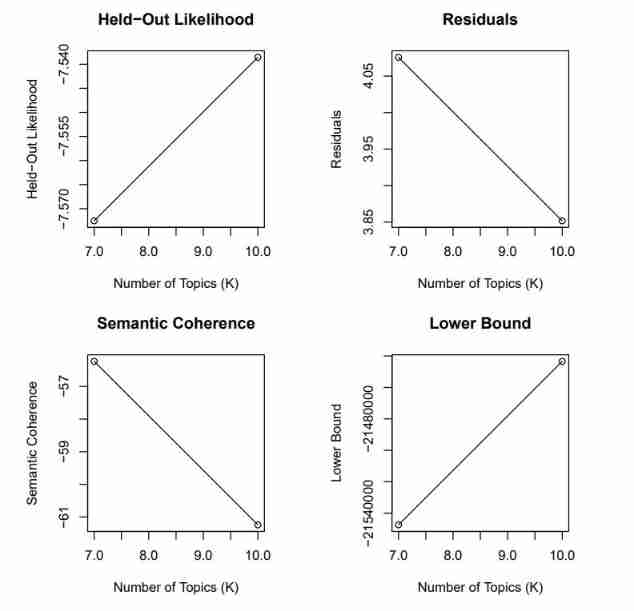
storage <- searchK(out$documents, out$vocab, K = c(7, 10), prevalence = ~rating + s(day), data = meta)

#  Visually select the number of topics with the help of chart visualization 
pdf("stm-plot-ntopics.pdf")
plot(storage)
dev.off()

#  Select the number of topics with the help of actual data 
t <- storage$out[[1]]
t <- storage$out[[2]]

Compare the number of two or more topics , By comparing semantic coherence SemCoh And exclusivity Exl Determine the appropriate number of topics

3.5 Understand: Interpreting the STM by plotting and inspecting results

After selecting the model , It is through stm Some functions provided in the package to show the results of the model . To keep consistent with the original paper , Use the initial model poliblogPrevFit As a parameter , Instead of SelectModel

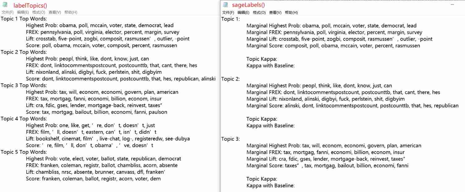
Sort the high-frequency words under each topic ：labelTopics()、sageLabels()

Both functions output words related to each topic , among sageLabels() Use only for models that contain content covariates . Besides ,sageLabels() Function result ratio labelTopics() A more detailed , By default, high-frequency words and other information under all topics are output

# labelTopics() Label topics by listing top words for selected topics 1 to 5.
labelTopicsSel <- labelTopics(poliblogPrevFit, c(1:5))
sink("output/labelTopics-selected.txt", append=FALSE, split=TRUE)
print(labelTopicsSel)
sink()

# sageLabels()  Than  labelTopics()  Output more detailed 
sink("stm-list-sagelabel.txt", append=FALSE, split=TRUE)
print(sageLabels(poliblogPrevFit))
sink()

TODO： The output results of the two functions are different

List documents that are highly relevant to a topic ：findthoughts()

shortdoc <- substr(out$meta$documents, 1, 200)
#  Parameters  'texts=shortdoc'  Means before outputting each document 200 Characters ,n Indicates the number of output related documents 
thoughts1 <- findThoughts(poliblogPrevFit, texts=shortdoc, n=2, topics=1)$docs[[1]]
pdf("findThoughts-T1.pdf")
plotQuote(thoughts1, width=40, main="Topic 1")
dev.off()

# how about more documents for more of these topics?
thoughts6 <- findThoughts(poliblogPrevFit, texts=shortdoc, n=2, topics=6)$docs[[1]]
thoughts18 <- findThoughts(poliblogPrevFit, texts=shortdoc, n=2, topics=18)$docs[[1]]
pdf("stm-plot-find-thoughts.pdf")
# mfrow=c(2, 1) The diagram will be output to 2 That's ok 1 In the table of columns 
par(mfrow = c(2, 1), mar = c(.5, .5, 1, .5))
plotQuote(thoughts6, width=40, main="Topic 6")
plotQuote(thoughts18, width=40, main="Topic 18")
dev.off()

Estimate metadata and topics / The relationship between topics ：estimateEffect

out$meta$rating<-as.factor(out$meta$rating)
# since we're preparing these coVariates by estimating their effects we call these estimated effects 'prep'
# we're estimating Effects across all 20 topics, 1:20. We're using 'rating' and normalized 'day,' using the topic model poliblogPrevFit. 
# The meta data file we call meta. We are telling it to generate the model while accounting for all possible uncertainty. Note: when estimating effects of one covariate, others are held at their mean
prep <- estimateEffect(1:20 ~ rating+s(day), poliblogPrevFit, meta=out$meta, uncertainty = "Global")
summary(prep, topics=1)
summary(prep, topics=2)
summary(prep, topics=3)
summary(prep, topics=4)

uncertainty Yes "Global", “Local”, "None" Three options ,The default is “Global”, which will incorporate estimation uncertainty of the topic proportions into the uncertainty estimates using the method of composition. If users do not propagate the full amount of uncertainty, e.g., in order to speed up computational time, they can choose uncertainty = “None”, which will generally result in narrower confidence intervals because it will not include the additional estimation uncertainty.

summary(prep, topics=1) Output results ：

Call:
estimateEffect(formula = 1:20 ~ rating + s(day), stmobj = poliblogPrevFit, 
    metadata = meta, uncertainty = "Global")


Topic 1:

Coefficients:
               Estimate Std. Error t value Pr(>|t|)    
(Intercept)    0.068408   0.011233   6.090 1.16e-09 ***
ratingLiberal -0.002513   0.002588  -0.971  0.33170    
s(day)1       -0.008596   0.021754  -0.395  0.69276    
s(day)2       -0.035476   0.012314  -2.881  0.00397 ** 
s(day)3       -0.002806   0.015696  -0.179  0.85813    
s(day)4       -0.030237   0.013056  -2.316  0.02058 *  
s(day)5       -0.026256   0.013791  -1.904  0.05695 .  
s(day)6       -0.010658   0.013584  -0.785  0.43269    
s(day)7       -0.005835   0.014381  -0.406  0.68494    
s(day)8        0.041965   0.016056   2.614  0.00897 ** 
s(day)9       -0.101217   0.016977  -5.962 2.56e-09 ***
s(day)10      -0.024237   0.015679  -1.546  0.12216    
---
Signif. codes:  0 ‘***’ 0.001 ‘**’ 0.01 ‘*’ 0.05 ‘.’ 0.1 ‘ ’ 1

3.6 Visualize: Presenting STM results

Summary visualization

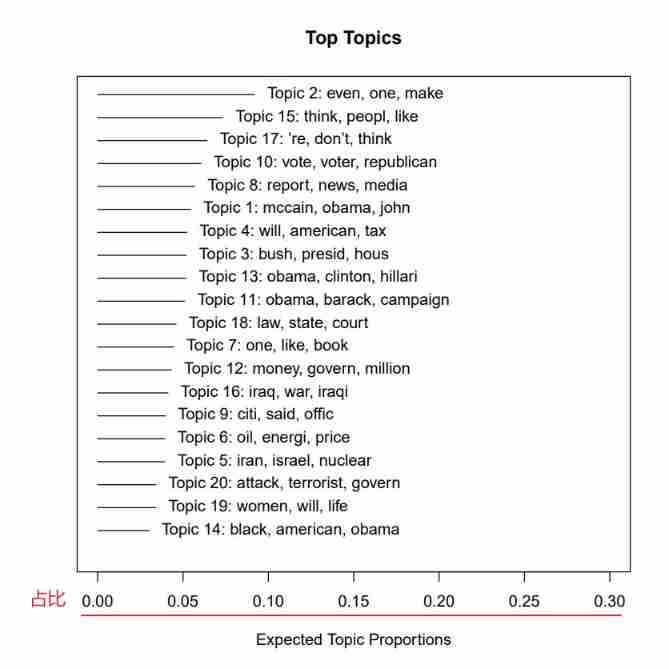
Topic proportion bar chart

# see PROPORTION OF EACH TOPIC in the entire CORPUS. Just insert your STM output
pdf("top-topic.pdf")
plot(poliblogPrevFit, type = "summary", xlim = c(0, .3))
dev.off()

Metadata/topic relationship visualization

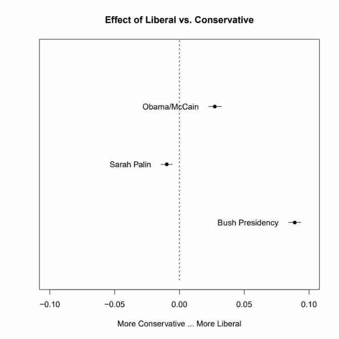
Topic relationship comparison diagram

pdf("stm-plot-topical-prevalence-contrast.pdf")
plot(prep, covariate = "rating", topics = c(6, 13, 18),
     model = poliblogPrevFit, method = "difference",
     cov.value1 = "Liberal", cov.value2 = "Conservative",
     xlab = "More Conservative ... More Liberal",
     main = "Effect of Liberal vs. Conservative",
     xlim = c(-.1, .1), labeltype = "custom",
     custom.labels = c("Obama/McCain", "Sarah Palin", "Bush Presidency"))
dev.off()

The theme 6、13、18 The custom label is "Obama/McCain"、“Sarah Palin”、“Bush Presidency”, The theme 6、 The theme 13 Our ideology is neutral , Neither conservative , Nor is it freedom , The theme 18 Our ideology tends to be conservative .

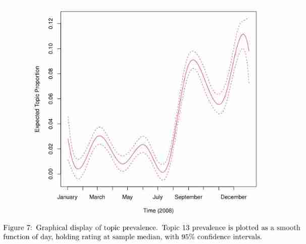
Trend chart of theme changing over time

pdf("stm-plot-topic-prevalence-with-time.pdf")
plot(prep, "day", method = "continuous", topics = 13, 
     model = z, printlegend = FALSE, xaxt = "n", xlab = "Time (2008)")
monthseq <- seq(from = as.Date("2008-01-01"), to = as.Date("2008-12-01"), by = "month")
monthnames <- months(monthseq)
# There were 50 or more warnings (use warnings() to see the first 50)
axis(1, at = as.numeric(monthseq) - min(as.numeric(monthseq)), labels = monthnames)
dev.off()

Operation error reporting , But you can output the following pictures , Unknown cause

topic content

Show which words in a topic are more relevant to one variable value and another variable value .

# TOPICAL CONTENT.
# STM can plot the influence of covariates included in as a topical content covariate.
# A topical content variable allows for the vocabulary used to talk about a particular 
# topic to vary. First, the STM must be fit with a variable specified in the content option.
# Let's do something different. Instead of looking at how prevalent a topic is in a class of documents categorized by meta-data covariate... 
# ... let's see how the words of the topic are emphasized differently in documents of each category of the covariate
# First, we we estimate a new stm. It's the same as the old one, including prevalence option, but we add in a content option
poliblogContent <- stm(out$documents, out$vocab, K = 20, 
                       prevalence = ~rating + s(day), content = ~rating, 
                       max.em.its = 75, data = out$meta, init.type = "Spectral")
pdf("stm-plot-content-perspectives.pdf")
plot(poliblogContent, type = "perspectives", topics = 10)
dev.off()

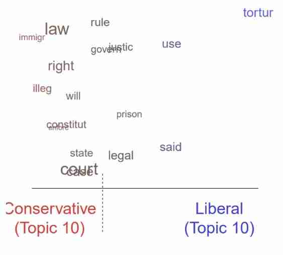
The theme 10 Related to Cuba . Its most commonly used word is “ detention 、 A jail sentence 、 court 、 illegal 、 cruel torture 、 Enforcement 、 Cuba ”. It shows the different views of liberals and conservatives on this theme , Liberals emphasize “ cruel torture ”, Conservatives stress “ illegal ” and “ law ” And other typical court language

original text ：Its top FREX words were “detaine, prison, court, illeg, tortur, enforc, guantanamo” Medium tortur Should be torture

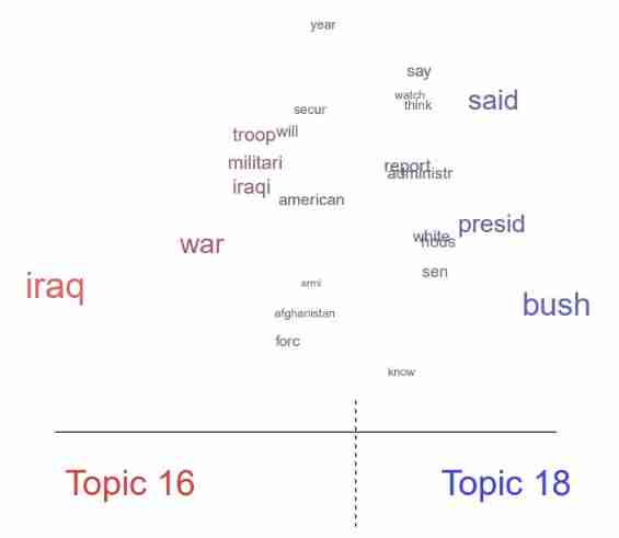
Draw lexical differences between topics

pdf("stm-plot-content-perspectives-16-18.pdf")
plot(poliblogPrevFit, type = "perspectives", topics = c(16, 18))
dev.off()

Plotting covariate interactions

# Interactions between covariates can be examined such that one variable may ??moderate??
# the effect of another variable.
###Interacting covariates. Maybe we have a hypothesis that cities with low $$/capita become more repressive sooner, while cities with higher budgets are more patient 
##first, we estimate an STM with the interaction
poliblogInteraction <- stm(out$documents, out$vocab, K = 20,
                           prevalence = ~rating * day, max.em.its = 75,
                           data = out$meta, init.type = "Spectral")
# Prep covariates using the estimateEffect() function, only this time, we include the 
# interaction variable. Plot the variables and save as pdf files.
prep <- estimateEffect(c(16) ~ rating * day, poliblogInteraction,
                       metadata = out$meta, uncertainty = "None")
pdf("stm-plot-two-topic-contrast.pdf")
plot(prep, covariate = "day", model = poliblogInteraction,
     method = "continuous", xlab = "Days", moderator = "rating",
     moderator.value = "Liberal", linecol = "blue", ylim = c(0, 0.12),
     printlegend = FALSE)
plot(prep, covariate = "day", model = poliblogInteraction,
     method = "continuous", xlab = "Days", moderator = "rating",
     moderator.value = "Conservative", linecol = "red", add = TRUE,
     printlegend = FALSE)
legend(0, 0.06, c("Liberal", "Conservative"),
       lwd = 2, col = c("blue", "red"))
dev.off()

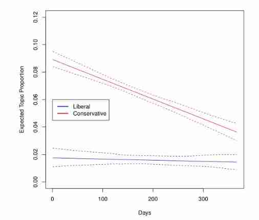
The figure above depicts the time （ Blog posting day ） And ratings （ Liberals and conservatives ） The relationship between . The theme 16 The prevalence is plotted as a linear function of time , The score is 0（ free ） or 1（ conservative ）.

3.7 Extend: Additional tools for interpretation and visualization

Draw a cloud of words

pdf("stm-plot-wordcloud.pdf")
cloud(poliblogPrevFit, topic = 13, scale = c(2, 0.25))
dev.off()

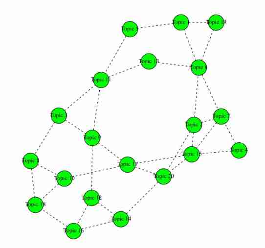
Topic relevance

# topicCorr().
# STM permits correlations between topics. Positive correlations between topics indicate
# that both topics are likely to be discussed within a document. A graphical network
# display shows how closely related topics are to one another (i.e., how likely they are
# to appear in the same document). This function requires 'igraph' package.
# see GRAPHICAL NETWORK DISPLAY of how closely related topics are to one another, (i.e., how likely they are to appear in the same document) Requires 'igraph' package
mod.out.corr <- topicCorr(poliblogPrevFit)
pdf("stm-plot-topic-correlations.pdf")
plot(mod.out.corr)
dev.off()

stmCorrViz

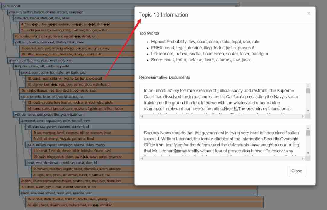
stmCorrViz software package Provides a different d3 Visual environment , This environment focuses on using hierarchical clustering methods to group topics , Thus visualizing topic relevance .

There is a garbled code problem

# The stmCorrViz() function generates an interactive visualisation of topic hierarchy/correlations in a structural topicl model. The package performs a hierarchical
# clustering of topics that are then exported to a JSON object and visualised using D3.
# corrViz <- stmCorrViz(poliblogPrevFit, "stm-interactive-correlation.html", documents_raw=data$documents, documents_matrix=out$documents)

stmCorrViz(poliblogPrevFit, "stm-interactive-correlation.html", 
           documents_raw=data$documents, documents_matrix=out$documents)

4 Changing basic estimation defaults

This section explains how to change stm The default setting in the estimation command of the package

First, we discuss how to choose among different methods of initializing model parameters , Then discuss how to set and evaluate convergence criteria , Then describe a method to accelerate convergence when analyzing documents containing tens of thousands or more , Last , Discuss some changes in the covariate model , These changes allow users to control the complexity of the model .

---

problem

ems.its and run What's the difference ？ems.its Group iterated algebra of representation , Every iteration run=20？

3.4-3 How to determine the appropriate number of topics according to the four diagrams ？

Add

stay Ingest part , The author mentioned other methods for text processing quanteda package , This package can easily import text and related metadata , Prepare the text to be processed , And convert the document into a document term matrix （document-term matrix）. Another bag ,readtext Contains very flexible tools , Used to read various text formats , Such as plain text 、XML and JSON Format , You can easily create a corpus from it .

To read data from other text handlers , You can use txtorg, This program can create three independent files ：a metadata file, a vocabulary file, and a file with the original documents. The default export format is LDA-C sparse matrix format, It can be used readCorpus() Set up "ldac"option To read

---

The paper ：stm: An R Package for Structural Topic Models (harvard.edu)

Reference article ：R Software STM package Practice - Bili, Bili (bilibili.com)

relevant github Warehouse ：

JvH13/FF-STM: Web Appendix - Methodology for Structural Topic Modeling (github.com)

dondealban/learning-stm: Learning structural topic modeling using the stm R package. (github.com)

bstewart/stm: An R Package for the Structural Topic Model (github.com)