当前位置:网站首页>PLC: automatically correct the data set noise, wash the data set | ICLR 2021 spotlight
PLC: automatically correct the data set noise, wash the data set | ICLR 2021 spotlight
2022-07-07 14:31:00 【VincentLee】
This paper proposes a more general feature-related noise category PMD, Based on this kind of noise, a data calibration strategy is constructed PLC To help the model converge better , Experiments on generated datasets and real datasets have proved the effectiveness of the algorithm . The scheme theory proposed in this paper is proved to be complete , It is very simple to apply , It's worth trying source : Xiaofei's algorithm Engineering Notes official account
The paper : Learning with Feature-Dependent Label Noise: A Progressive Approach
- Address of thesis :https://arxiv.org/abs/2103.07756v3
- Paper code :https://github.com/pxiangwu/PLC
Introduction
In large datasets , Due to the ambiguity of the label and the carelessness of the annotator , Wrong annotation is inevitable . Because noise has a great impact on supervised training , So it is very important to study how to deal with wrong annotation in practical application .
Some classical methods carry out independent and identically distributed noise (i.i.d.) Assumptions , It is considered that noise has nothing to do with data characteristics , It has its own rules . These methods either directly predict the noise distribution to distinguish the noise , Or introduce additional regular terms / Loss term to distinguish noise . Other methods prove , The commonly used loss term itself can resist these independent and identically distributed noises , Don't care .
Although these methods have theoretical guarantee , But in reality, the performance is poor , Because the assumption of independent and identically distributed noise is not true . It means , The noise of the data set is diverse , And it is related to data characteristics , For example, a fuzzy cat may be mistaken for a dog . In case of insufficient light or blocking , The picture has lost important visual discrimination clues , It is easy to be mislabeled . In order to meet this real challenge , Dealing with noise requires not only effective , Its versatility is also very necessary .
SOTA Most methods use data recalibration (data-recalibrating) Strategies to adapt to a variety of data noise , This strategy gradually confirms the trusted data or gradually corrects the label , Then use these data for training . As data sets become more accurate , The accuracy of the model will gradually improve , Finally, it converges to high accuracy . This strategy makes good use of the learning ability of deep network , Get good results in practice .
But at present, there is no complete theoretical proof of the internal mechanism of these strategies , Explain why these strategies can make the model converge to the ideal state . This means that these strategies are case by case Of , Super parameters need to be adjusted very carefully , Difficult to be universal .
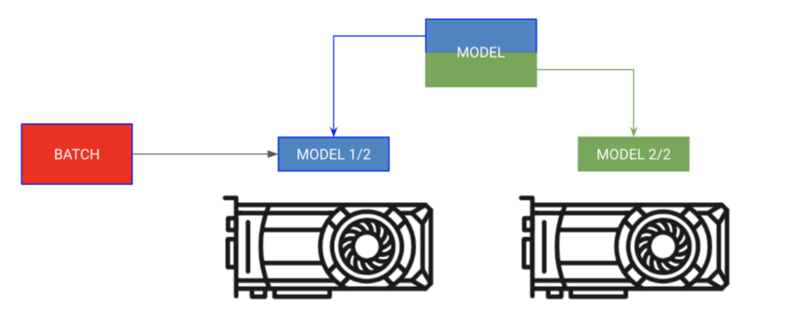
Based on the above analysis , The paper defines the more common PMD Noise family (Polynomial Margin Dimishing Noise Family), Contains any type of noise except obvious errors , More in line with the real scene . be based on PMD Noise family , This paper proposes a data calibration method with theoretical guarantee , The labels of the data are calibrated step by step according to the confidence of the noise classifier . Flow chart 1 Shown , Start with high confidence data , Use the prediction results of the noise classifier to calibrate these data , Then use the calibrated data to improve the model , Carry out label calibration and model upgrading alternately until the model converges .
Method
First define some mathematical symbols , Take the two category task as an example :
- Define feature space $\mathcal{X}$, data $(x,y)$ From the distribution $D=\mathcal{X}\times{0,1}$ From sampling .
- Definition $\eta(x)=\mathbb{P}y=1|x$ It's a posterior probability , The higher the value, the more obvious the positive label is , The smaller the value, the more obvious the negative label .
- Define the noise function $\tau{0,1}(x)=\mathbb{P}=\tilde{y}=1 | y=0, x$ and $\tau{1,0}(x)=\mathbb{P}=\tilde{y}=0 | y=1, x$, among $\tilde{y}$ Label for errors . Hypothetical data $x$ The real label is $y=0$, Then there are $\tau_{0,1}(x)$ Probability is incorrectly labeled 1.
- Definition $\tilde{\eta}(x)=\mathbb{P}\tilde{y}=1|x$ Is the posterior probability of noise .
- Definition $\eta^{*}(x)=\mathbb{I}_{\eta(x)\ge\frac{1}{2}}$ Bayesian optimal classifier , When A To true $\mathbb{I}_A=1$, Otherwise 0.
- Definition $f(x):\mathcal{X}\to 0,1$ Scoring function for classifier , It's usually online softmax Output .
Poly-Margin Diminishing Noise
PMD Noise is only a function of noise $\tau$ Bound to a specific $\eta(x)$ Middle zone , Noise function in the region $\tau$ It doesn't matter how much it's worth . This form can not only cover feature independent scenes , It can also be generalized to some specific scenes of previous noise research .
PMD The definition of noise is shown above ,$t0$ It can be considered as the space between the left and right (margin).PMD Conditions only require $\tau$ The upper bound of is polynomial and monotonically decreases in the confidence region of Bayesian classifier , and $\tau{0,1}(x)$ and $\tau_{1,0}(x)$ stay ${ x:|\eta(x)-\frac{1}{2}| < t_0 }$ Any value in the area .
Ahead PMD Noise description may be abstract , The paper provides visual pictures to help you understand :
- chart a It is the result of Bayesian optimal classifier , That is, the correct label . From below $\eta(x)$ The curve shows , The binary classification probability of the data on both sides is quite different , It is easy to distinguish . The binary classification probability of the intermediate data is relatively close , There is a great possibility of mismarking , That's what we need to focus on .
- chart b It's uniform noise , The noise considers that the misclassification probability is independent of the characteristics , Every data point has the same probability of being misclassified . The black in the above figure is the data that is considered to be correct , Red is the data considered as noise , You can see , After uniform noise treatment , The data distribution is chaotic .
- chart c yes BCN noise , The noise value increases with $\eta^{}(x)$ The confidence of . As can be seen from the above figure , The processed noise data basically fall in the middle area , That is, where it is easy to be mistaken . But because of BCN The boundary of noise and $\eta^{}(x)$ Highly correlated , In practice, we usually use the output of the model to approximate $\eta^{*}(x)$, Obviously, there will be a big difference in the scene with a high degree of noise .
- chart d yes PMD noise , Constrain the noise in $\eta^{*}(x)$ In the middle of , The noise value in the area is arbitrary . The advantage of doing so is , Different noise levels can be dealt with by adjusting the size of the area , As long as it's not an obvious mistake ( That is to say $\eta$ The higher and lower parts are marked incorrectly ) apply . As can be seen from the above figure , The processed clean data is basically distributed on both sides , That is, where I believe .
The Progressive Correction Algorithm
be based on PMD noise , The paper proposes to train and correct labels step by step PLC(Progressive Label Correction) Algorithm . The algorithm first uses the original data set warm-up Stage training , Get a preliminary network that has not been fitted with noise . next , Use warm-up The preliminary network obtained corrects the labels of high confidence data , The paper holds that ( The theory also proves ) Noise classifier $f$ High confidence prediction can be compared with Bayesian optimal classifier $\eta^{*}$ bring into correspondence with .
When correcting labels , First select a high threshold $\theta$. If $f$ Forecast label and label $\tilde{y}$ Different and the prediction confidence is higher than the threshold , namely $|f(x)-1/2|>\theta$, Will $\tilde{y}$ Corrected to $f$ The forecast tab . Repeat the label correction and retrain the model with the corrected data set , Until no labels are corrected .
next , Lower the threshold slightly $\theta$, Repeat the above steps with the reduced threshold , Until the model converges . In order to facilitate the later theoretical analysis , This paper defines a continuously increasing threshold $T$, Give Way $\theta=1/2-T$, Specific logic such as Algorithm 1 Shown .
- Generalizing to the multi-class scenario The above descriptions are all binary scenes , In a multi category scenario , First define $fi(x)$ Label for classifier $i$ The probability of prediction ,$h_x=argmax_if_i(x)$ Tags predicted for the classifier . take $|f(x)-\frac{1}{2}|$ The judgment of is modified as |$f{hx}(x)-f{\tilde{y}}(x)|$, When the result is greater than the threshold $\theta$ when , Label $\tilde{y}$ Change to label $h_x$. In the process of practice , Adding logarithm to the difference judgment will be more robust .
Analysis
This is the core of the paper , Mainly from the theoretical point of view to verify the universality and correctness of the proposed method . We won't go on here , If you are interested, please go to the original , We only need to know the usage of this algorithm .
Experiment
At present, there is no public data set for the noise problem of data sets , So we need to generate data sets for experiments , This paper is mainly about CIFAR-10 and CIFAR-100 Data generation and experiment on . First train a network on the original data , The prediction probability of the network is used to approximate the real posterior probability $\eta$. be based on $\eta$ Resample data $x$ The label of $y_x\sim\eta(x)$ As a clean data set , The previously trained network is used as the Bayesian optimal classifier $\eta^{*}:\mathcal{X}\to{1,\cdots,C}$, among $C$ Is the number of categories . It should be noted that , In multi category scenarios ,$\eta(x)$ Output as vector ,$\eta_i(x)$ The number of the corresponding vector $i$ Elements .
For the generation of noise , There are characteristic correlation noise and independent identically distributed noise (i.d.d) Two kinds of :
- For feature related noise , In order to increase the challenge of noise , Every data $x$ According to the noise function, it is possible to classify from the highest confidence $ux$ Become the second confidence classification $s_x$, Where the noise function and $\eta(x)$ Probability Correlation .$s_x$ about $\eta^{*}(x)$ It is the category with the highest degree of confusion , It can most affect the performance of the model . in addition , because $y_x$ It's from $\eta(x)$ From sampling , It is the category with the highest confidence , So it can be considered that $y_x$ Namely $u_x$. Overall speaking , For data $x$, When generating data, it either becomes $s_x$, Or keep $u_x$. There are three kinds of feature related noise PMD Noise function in noise family : Is the noise function $\tau{u_x,s_x}$ Add a constant factor , Make the final noise ratio meet the expectations . about PMD noise ,35% and 70% The noise level of represents 35% and 70% The clean data of is modified into noise .
- Independent identically distributed noise by constructing noise transformation matrix $T$ To modify the label , among $T{ij}=P(\tilde{y}=j|y=i)=\tau{ij}$ For real labels $y=i$ Convert to label $j$ Probability . For the label $i$ The data of , Change its label to from matrix $T$ Of the $i$ Labels sampled from the probability distribution of rows . This paper adopts two kinds of common independent identically distributed noise :1) Uniform noise (Uniform noise), Real label $i$ The probability of converting to other tags is the same , namely $T{ij}=\tau/(C-1)$, among $i\ne j$,$T{ii}=1-\tau$,$\tau$ Is the noise level .2) Asymmetric noise (Asymmetric noise), Real label $i$ There is a probability $T{ij}=\tau$ Probability is converted into labels $j$, or $T{ii}=1-\tau$ The probability remains the same .
In the experiment , Some experiments will combine feature related noise and independent identically distributed noise to generate and experiment noise data sets , The final verification standard is the accuracy of the model on the verification set . During training , use 128 batch size、0.01 Learning rate and SGD Optimizer , Co training 180 Period guarantees convergence , repeat 3 Take the mean and standard deviation for the second time .
PMD Noise test , stay 35% and 70% Performance comparison under noise level .
Mixed noise test , stay 50%-70% Performance comparison under noise level .
Superparametric comparative experiment .
Performance comparison on real data sets .
Conclusion
This paper proposes a more general feature-related noise category PMD, Based on this kind of noise, a data calibration strategy is constructed PLC To help the model converge better , Experiments on generated datasets and real datasets have proved the effectiveness of the algorithm . The scheme theory proposed in this paper is proved to be complete , It is very simple to apply , It's worth trying .
边栏推荐
- 小米的芯片自研之路
- Equipment failure prediction machine failure early warning mechanical equipment vibration monitoring machine failure early warning CNC vibration wireless monitoring equipment abnormal early warning
- 寺岗电子称修改IP简易步骤
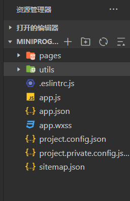
- 小程序目录结构
- IP address home location query full version
- Excuse me, I have three partitions in Kafka, and the flinksql task has written the join operation. How can I give the join operation alone
- Small game design framework
- C # switch pages through frame and page
- libSGM的horizontal_path_aggregation程序解读
- 数据湖(九):Iceberg特点详述和数据类型
猜你喜欢


随机推荐
潘多拉 IOT 开发板学习(HAL 库)—— 实验12 RTC实时时钟实验(学习笔记)
Mlgo: Google AI releases industrial compiler optimized machine learning framework
Ascend 910实现Tensorflow1.15实现LeNet网络的minist手写数字识别
docker部署oracle
属性关键字OnDelete,Private,ReadOnly,Required
Codes de non - retour à zéro inversés, codes Manchester et codes Manchester différentiels couramment utilisés pour le codage des signaux numériques
Beginner JSP
LeetCode 648. Word replacement
MRS离线数据分析:通过Flink作业处理OBS数据
Hangdian oj2092 integer solution
Equipment failure prediction machine failure early warning mechanical equipment vibration monitoring machine failure early warning CNC vibration wireless monitoring equipment abnormal early warning
gvim【三】【_vimrc配置】
低代码平台中的数据连接方式(下)
Search engine interface
PERT图(工程网络图)
Differences between cookies and sessions
Multi merchant mall system function disassembly lecture 01 - Product Architecture
JS image to Base64
Excuse me, I have three partitions in Kafka, and the flinksql task has written the join operation. How can I give the join operation alone
PD虚拟机教程:如何在ParallelsDesktop虚拟机中设置可使用的快捷键?