当前位置:网站首页>Data analysis Seaborn visualization (for personal use)
Data analysis Seaborn visualization (for personal use)
2022-07-06 03:27:00 【Up and down black】
Reference Content
【Python】 An hour will take you to master seaborn visualization _ Bili, Bili _bilibili
Catalog
2、 Observe the distribution of variables
3、figure-level functions have FacetGrid characteristic
Two 、 Relationship analysis of numerical variables
2、sns.lmplot(): Analyze the linear relationship between two variables
3、sns.displot(): Plot the joint distribution of two variables
4、sns.jointplot(): Plot the joint distribution and respective distribution of two variables
(2)jointplot Upgraded version :JointGrid, It can be done by g.plot Custom function
(3)sns.pairplot(): Plot the joint distribution of all numerical variables in pairs
(4)pairplot Upgraded version :PairGrid, It can be done by g.map Custom function
(5)data.corr()+sns.heatmap(): Plot the correlation coefficients of all numerical variables in pairs
3、 ... and 、 Analysis of category variables
1、 Distribution of category variables :sns.countplot(), similar sns.histplot()
2、 The relationship between category variables and numerical variables
(2) The value range of numerical variables in different categories :boxplot, boxenplot
Four 、FacetGrid, PairGrid Custom drawing function in
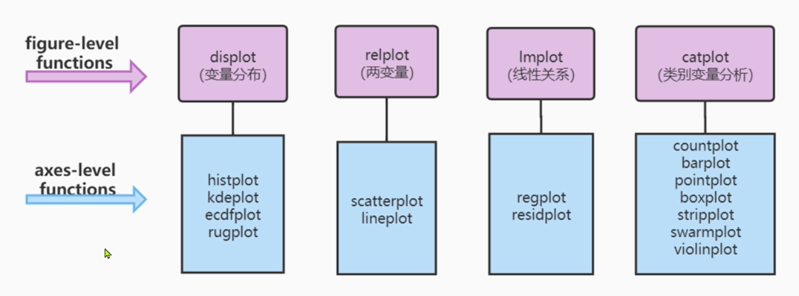
seaborn The function structure of can usually be divided into : Figure drawing function ( Purplish red ) And axis drawing function ( sky blue ).
Each kind of graph drawing function aggregates the functions of the corresponding axis drawing function , It also provides corresponding interfaces .
One 、 Variable distribution
Get a data , First, check the distribution of variables :
- Variable value range , Whether there are outliers (outliers)?
- Whether the distribution of variables is approximately normal ? If not , Is there any offset ? Is there a bimodal distribution (bimodality)?
- If the data set is divided according to category variables , Whether the distribution of variables on each subset is very different ?
1、 View outliers
(1) use seaborn Data set included in
print(sns.get_dataset_names())
penguin_df = sns.load_dataset('penguins')
penguin_df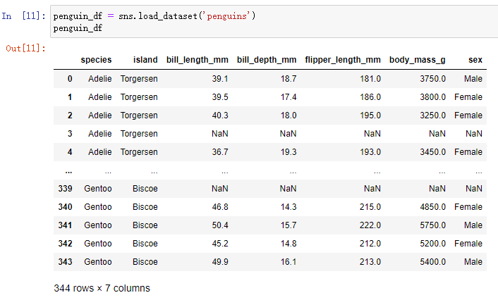
(2)sns.boxplot(): View the value range of numeric variables , Observe whether there are abnormal values ( Box figure )
sns.boxplot(data=penguin_df, x='bill_length_mm') # Define data and variable names 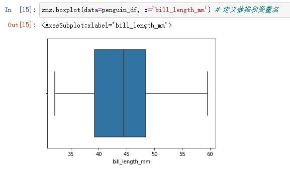
In the figure The line in the middle of the box is the median of the data ; The left and right boundaries of the box are quartiles (75% The value of is less than 49 Of ,25% The value is less than 39); The two lines outside the box represent the maximum and minimum values within a reasonable range ( Calculated by formula ), Beyond this range , The data is unreasonable , It may be an outlier , It needs to be analyzed in detail .
1、boxplot Corresponding catplot( Category variable analysis ), therefore Box diagram It can also be used. catplot draw :
sns.catplot(data=penguin_df, x='bill_length_mm',kind='box') # Need to define kind
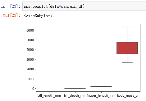
2、 You can also put the box diagram of all variables into one diagram , But the effect is often not good because the data is not an order of magnitude :
sns.boxplot(data=penguin_df)

(3) Observe outliers
sns.boxplot(data=tip_df)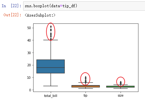
The red circle in the figure may be the point of outliers ( Specific analysis of specific problems ).
2、 Observe the distribution of variables
(1)sns.displot(): View the distribution of variables
sns.displot(data=penguin_df, x='bill_length_mm') 
#  By setting bins To control the division of histogram
sns.displot(data=penguin_df, x='bill_length_mm', bins=50)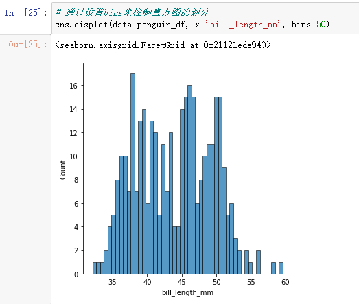
bins If the division is too rough, the distribution characteristics of the data may be ignored , But sometimes too detailed division will lead to excessive interpretation . You can see that the above figure shows a bimodal distribution .
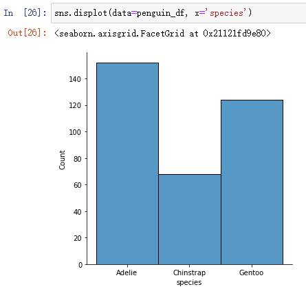
1、displot Category variables can also be analyzed :
sns.displot(data=penguin_df, x='species')
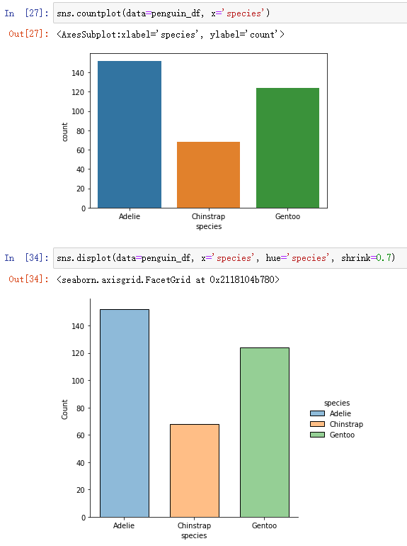
2、 Contrast with countplot Analyze category variables :
sns.countplot(data=penguin_df, x='species')sns.displot(data=penguin_df, x='species', hue='species', shrink=0.7)displot Can pass hue Parameter to distinguish colors , adopt shink Zoom the histogram
(2)sns.displot(): see kde curve
Use kernel function to fit the distribution of data , Gaussian kernel function is used by default .
- Method 1 :
sns.displot(data=penguin_df, x='bill_length_mm', kind='kde')- Method 2 :
sns.kdeplot(data=penguin_df, x='bill_length_mm')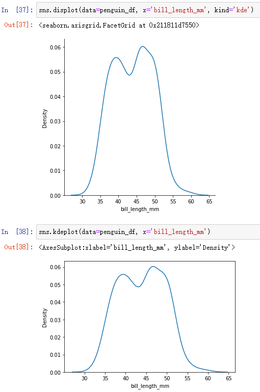
rugplot It doesn't take up space , It can be directly superimposed on displot On the image of :
sns.displot(data=penguin_df, x='bill_length_mm', kind='kde', rug=True) 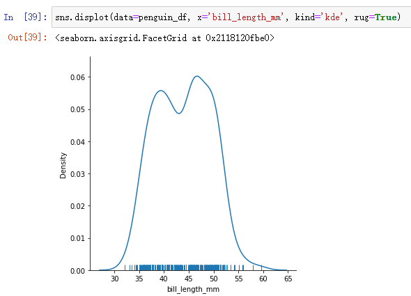
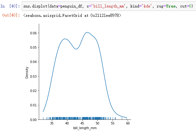
although kde The curve is easier to observe the distribution of data , However, the drawing at the edge of the image may exceed the value range .
- Solution 1 :( Make cut=0)
sns.displot(data=penguin_df, x='bill_length_mm', kind='kde', rug=True, cut=0)
But this method may change the data distribution .
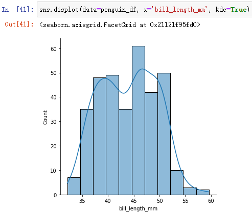
- Solution 2 :( Overlay and draw on the histogram kde)
sns.displot(data=penguin_df, x='bill_length_mm', kde=True)
(3) Analyze bimodal distribution
sns.displot(data=penguin_df, x='bill_length_mm', kind='kde', hue='species')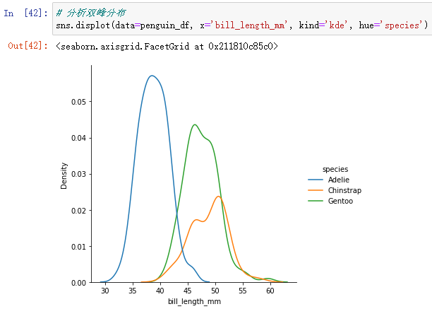
As you can see from the diagram , Penguins are the longest in different species kde The distribution is different , There is a certain gap between them . Therefore, the superposition will show the characteristics of bimodal distribution .
(4) Analyze the offset
Data can be processed logarithmically
(5) Empirical distribution function (acdfplot)
sns.displot(data=penguin_df, x='bill_length_mm', kind='ecdf') 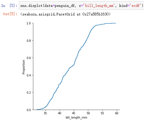
In the figure 55 The corresponding proportion is 0.97, Indicates that the data is lower than 55 The data accounts for 75%. The function is similar to the box diagram , It's just shown in different forms .
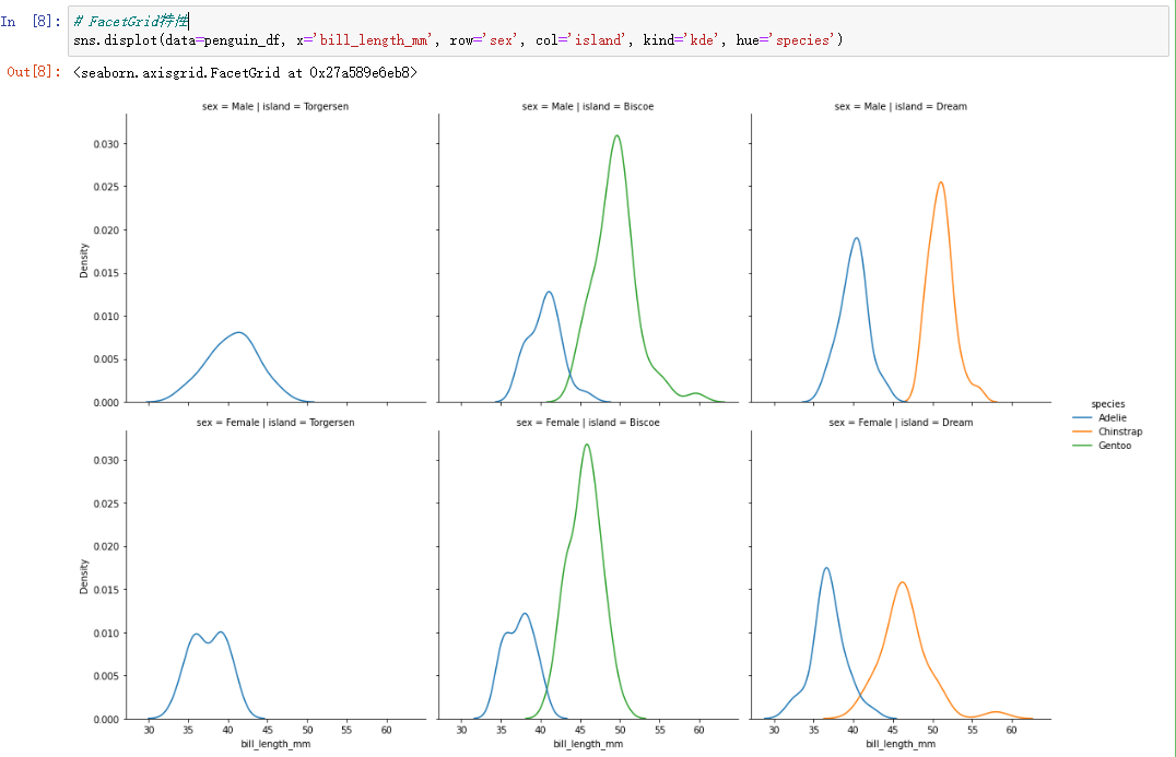
3、figure-level functions have FacetGrid characteristic
FacetGrid Set rows and columns as category variables , According to different categories of data variables , Divide the data into different subsets , Analyze the distribution of each variable on each subset .( It is equivalent to plotting the conditional probability distribution of variables )
sns.displot(data=penguin_df, x='bill_length_mm', row='sex', col='island', kind='kde', hue='species')Set the row to gender ( There are two categories ), The column is set to island ( There are three categories ), Draw penguins with long mouths kde curve (bill_length_mm).
Two 、 Relationship analysis of numerical variables
1、sns.relplot():
- Draw a scatter plot
sns.relplot(data=tip_df, x='total_bill', y='tip', hue='time', style='time', markers=['o', '^'])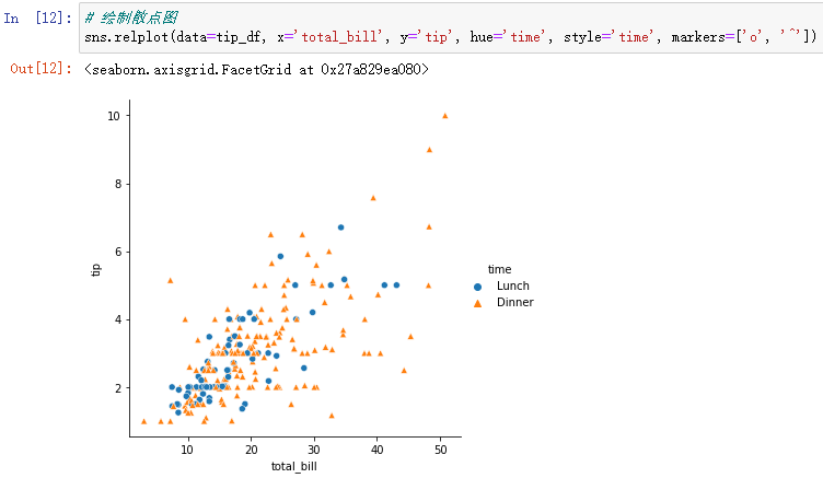
markers You can customize the style of the point in the diagram
sns.relplot(data=tip_df, x='total_bill', y='tip', hue='size', size='size') 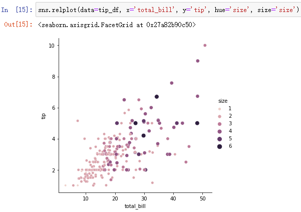
When there are many categories , Will use progressive colors , adopt size You can also set the size .
- Draw wiring diagram
sns.relplot(data=tip_df, x='total_bill', y='tip',kind='line') 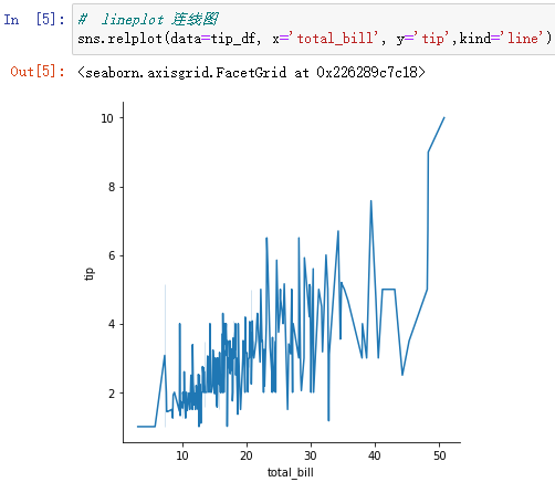
The picture above is a little messy , Because the connection diagram is suitable for analyzing time series data 、 Fluctuation of stock price, etc .
#  Stock price analysis
stock_df = pd.DataFrame(dict(time=np.arange(500), price=np.random.randn(500).cumsum()+np.ones(500)*50))
sns.relplot(data=stock_df, x='time', y='price', kind='line')
Random number generation 500 Number , Use the cumulative sum function (cumsum) Achieve the effect of continuous change to simulate the change of stock price .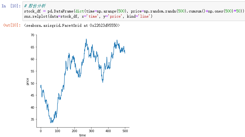
2、sns.lmplot(): Analyze the linear relationship between two variables
Front facing tip_df When plotting the scatter diagram, you can see that the data has a certain correlation , So you can use lmplot Draw the regression line .
sns.lmplot(data=tip_df, x='total_bill', y='tip') 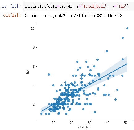
regplot and lmplot The effect of drawing regression line is the same :
sns.regplot(data=tip_df, x='total_bill', y='tip') 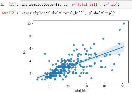
adopt residplot Draw a residual diagram :
sns.residplot(data=tip_df, x='total_bill', y='tip') 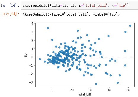
In a rational way ( If it fits well ), The residuals should be randomly distributed , The residual here also shows a certain divergence distribution , It must be that the relationship between the two variables has not been excavated .
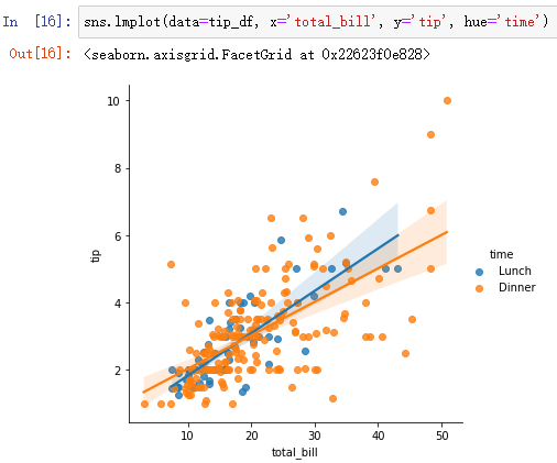
- lmplot Can also be combined with relplot Add category variables as well
sns.lmplot(data=tip_df, x='total_bill', y='tip', hue='time')
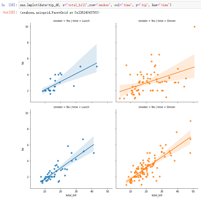
- lmplot Also has the FacetGrid characteristic
sns.lmplot(data=tip_df, x='total_bill',row='smoker', col='time', y='tip', hue='time')
3、sns.displot(): Plot the joint distribution of two variables
Histogram form :
sns.displot(data=penguin_df, x='bill_length_mm', y='bill_depth_mm')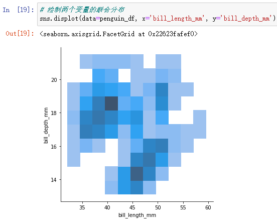
kde Curve form :
sns.displot(data=penguin_df, x='bill_length_mm', y='bill_depth_mm', kind='kde')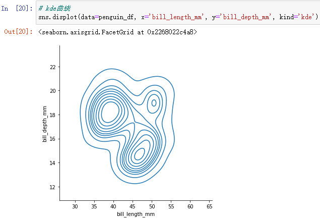
Can be set by thresh(0-1) To control the range of graphic display 、level Control the density of the line .
It can also be used. displot Draw the joint distribution of category variables :
sns.displot(data=penguin_df, x='island', y='species')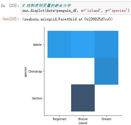
As you can see from the diagram ,Gentoo Only in Biscore island On , stay Biscore island On ,Gentoo Make up the majority , But there are still some Adelie.
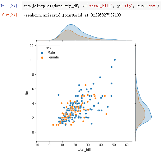
4、sns.jointplot(): Plot the joint distribution and respective distribution of two variables
(1)sns.jointplot()
By default , The joint distribution is a scatter , Can pass kind Set it up .`kind` is one of ['scatter', 'hist', 'hex', 'kde', 'reg', 'resid']
sns.jointplot(data=tip_df, x='total_bill', y='tip') 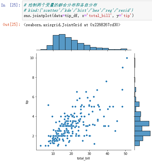
You can also use hue Add a category variable :
And displot identical ,jointplot You can also plot two category variables .
(2)jointplot Upgraded version :JointGrid, It can be done by g.plot Custom function
g = sns.JointGrid(data=tip_df, x='total_bill', y='tip')
g.plot(sns.histplot, sns.boxplot) # Use histogram in the middle , Box drawing for edge 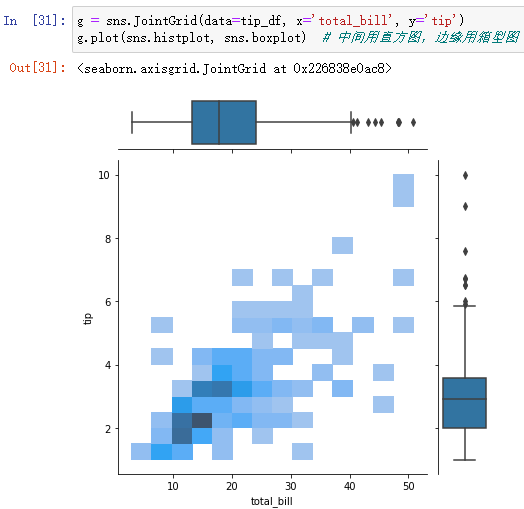
The customized part can also be more specific :
g = sns.JointGrid(data=tip_df, x='total_bill', y='tip')
g.plot_joint(sns.kdeplot)  #  Joint distribution
g.plot_marginals(sns.histplot, kde=True) # The distribution of the edges 
(3)sns.pairplot(): Plot the joint distribution of all numerical variables in pairs
sns.pairplot(data=tip_df, kind='kde')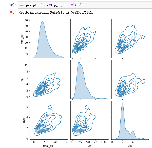
When there are many variables , You can choose the key variables you need for analysis :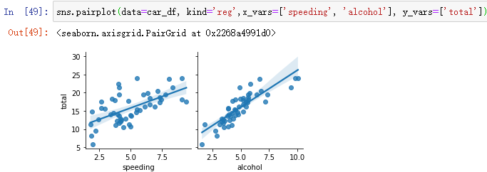
(4)pairplot Upgraded version :PairGrid, It can be done by g.map Custom function
g = sns.PairGrid(data=car_df, x_vars=['total', 'speeding', 'alcohol'], y_vars=['total', 'speeding', 'alcohol'])
g.map_upper(sns.scatterplot)
g.map_diag(sns.histplot, kde=True)
g.map_lower(sns.regplot)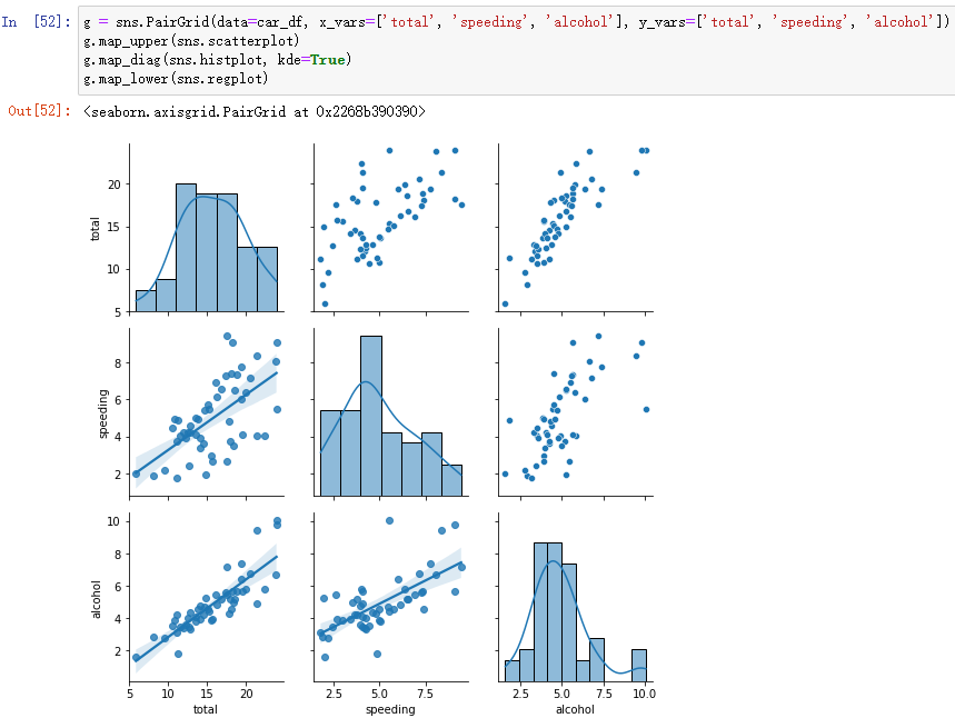
(5)data.corr()+sns.heatmap(): Plot the correlation coefficients of all numerical variables in pairs
First, find the correlation coefficient of each pair of variables :
car_cor = car_df.corr()
car_cor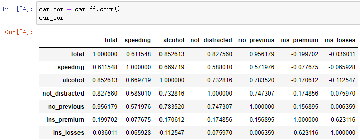 Then the obtained correlation coefficient is expressed in the form of thermodynamic diagram :
sns.heatmap(car_cor, cmap='Blues', annot=True, fmt='.2f', linewidth=0.5)
among annot Used to display values ,fmt='.2f' Represents a floating point type , Keep to two decimal places .
3、 ... and 、 Analysis of category variables
1、 Distribution of category variables :sns.countplot(), similar sns.histplot()
sns.catplot(data=tip_df, x='time', kind='count')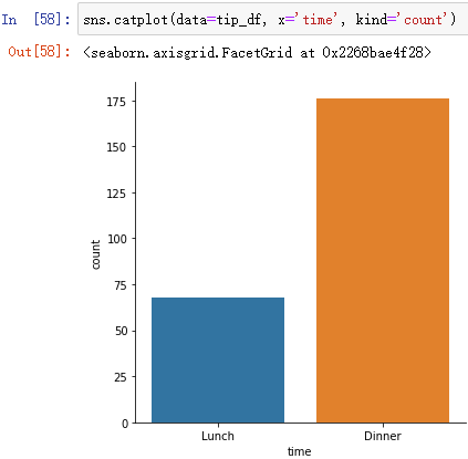
2、 The relationship between category variables and numerical variables
(1) The mean value of numerical variables in different categories / Median estimate :barplot, pointplot
sns.catplot(data=penguin_df, x='species', y='bill_length_mm', kind='bar', estimator=np.median, hue='island')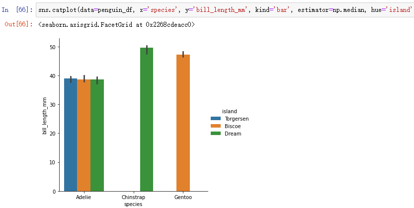
sns.catplot(data=penguin_df, x='species', y='bill_length_mm', kind='point') 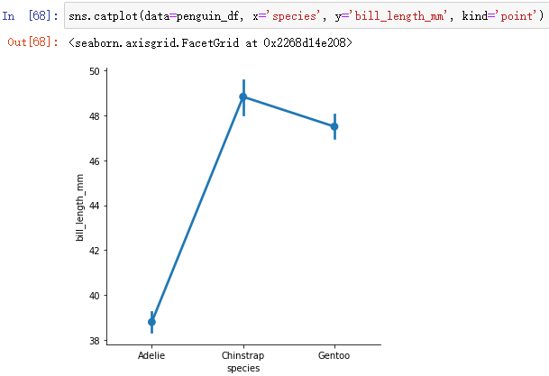
(2) The value range of numerical variables in different categories :boxplot, boxenplot
sns.catplot(data=penguin_df, x='species', y='bill_length_mm', kind='box') 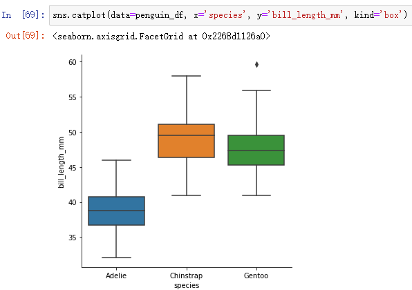
In general boxplot That's enough. , When the variable value range is large , It can be used boxenplot( For big data sets ).boxenplot You can draw a box diagram step by step .
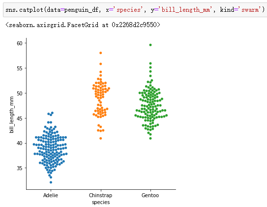
(3) Distribution diagram of numerical variables in different categories :stripplot, swarmplot, violinplot
The strip chart combines the characteristics of scatter chart and histogram :
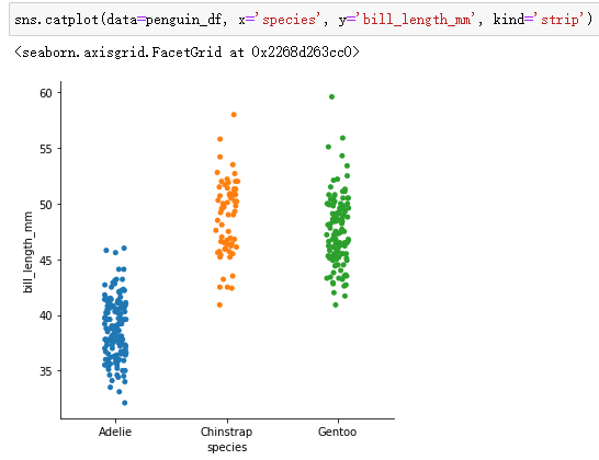
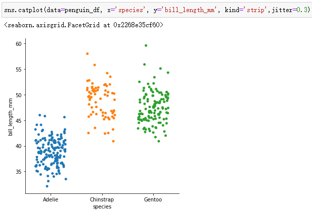
sns.catplot(data=penguin_df, x='species', y='bill_length_mm', kind='strip',jitter=0.3)adopt jitter You can set the width of the strip chart , Value range [0,1]
swarmplot:
violinplot:
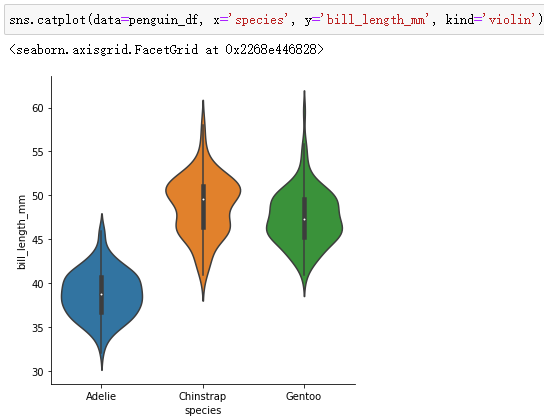
Can be swarmplot Overlay to violinplot On :
sns.catplot(data=penguin_df, x='species', y='bill_length_mm', kind='violin')
sns.swarmplot(data=penguin_df, x='species', y='bill_length_mm', color='w') #  Here want to use axes-level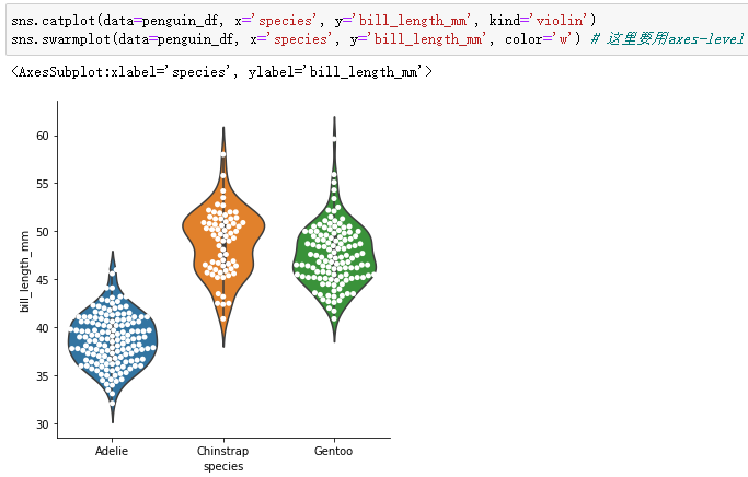
Four 、FacetGrid, PairGrid Custom drawing function in
1、FacetGrid
g = sns.FacetGrid(data=tip_df, row='time', col='smoker')  #  The defined rows and columns need to be category changed ; The picture is only framed
#  Custom part
g.map(sns.kdeplot, 'tip')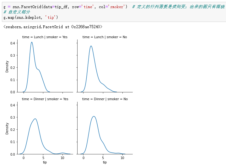
Plot the joint distribution
g = sns.FacetGrid(data=tip_df, row='time', col='smoker')
#  You can also plot the joint distribution of two variables
g.map(sns.scatterplot,'total_bill', 'tip')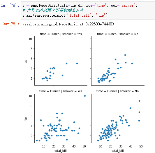
2、PairGrid
Usage and pairplot similar
g = sns.PairGrid(data=penguin_df,hue='species')
g.map_diag(sns.kdeplot)
g.map_offdiag(sns.scatterplot)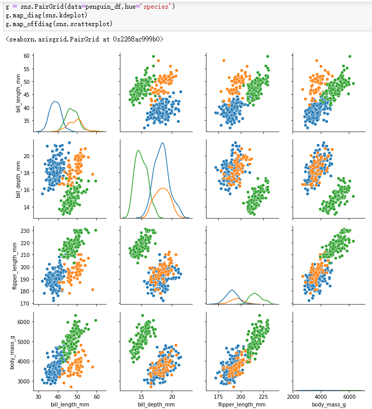
边栏推荐
- Pytorch基础——(2)张量(tensor)的数学运算
- Quartz misfire missed and compensated execution
- Advanced learning of MySQL -- Fundamentals -- isolation level of transactions
- Shell 传递参数
- Recommended foreign websites for programmers to learn
- Idea push rejected solution
- 2.2 STM32 GPIO operation
- 3.2 rtthread 串口设备(V2)详解
- 遥感图像超分辨率论文推荐
- 1.16 - check code
猜你喜欢
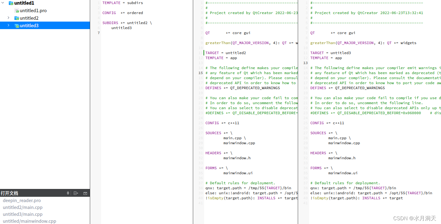
多项目编程极简用例
Mysqldump data backup

Exness foreign exchange: the governor of the Bank of Canada said that the interest rate hike would be more moderate, and the United States and Canada fell slightly to maintain range volatility
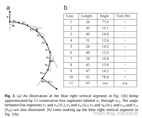
EDCircles: A real-time circle detector with a false detection control 翻译
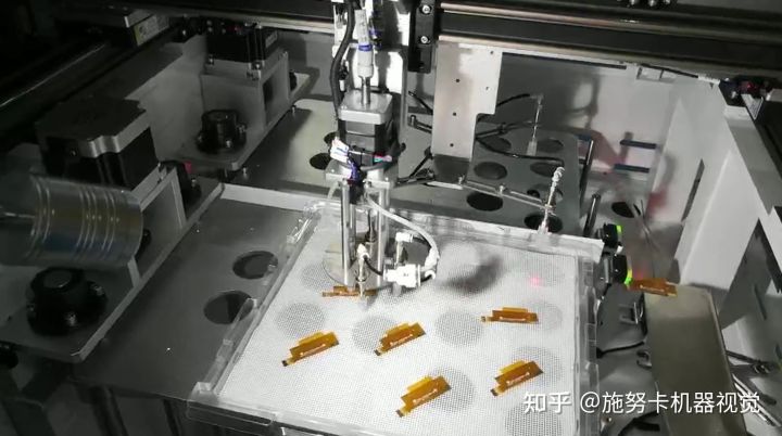
施努卡:视觉定位系统 视觉定位系统的工作原理
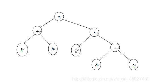
BUAA计算器(表达式计算-表达式树实现)

three.js网页背景动画液态js特效
Problems encountered in 2022 work IV
Teach you to build your own simple BP neural network with pytoch (take iris data set as an example)
2022工作中遇到的问题四
随机推荐
八道超经典指针面试题(三千字详解)
How to do function test well
Eight super classic pointer interview questions (3000 words in detail)
MPLS experiment
深入刨析的指针(题解)
three.js网页背景动画液态js特效
Buuctf question brushing notes - [geek challenge 2019] easysql 1
银行核心业务系统性能测试方法
Cubemx 移植正点原子LCD显示例程
Linear regression and logistic regression
Record the process of reverse task manager
Audio audiorecord binder communication mechanism
Quartz misfire missed and compensated execution
jsscript
2.2 STM32 GPIO操作
教你用Pytorch搭建一个自己的简单的BP神经网络( 以iris数据集为例 )
3.2 rtthread 串口设备(V2)详解
Restful style
Selenium share
深入探究指针及指针类型