当前位置:网站首页>History of object recognition
History of object recognition
2022-07-06 09:53:00 【zyw2002】
stay github I see a very good picture summarized on ( Original image address ) Code first
Overview of object recognition
The development history :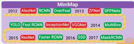
Image classification (Image Classification)
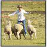
Mission : Classify the images according to the dominant objects in the images .
Data sets :MNIST, CIFAR, ImageNet
Object positioning (Object Localization)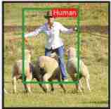
Mission : Predict the image area containing the dominant target . Then we use image classification to recognize the target in this area .
Data sets :ImageNet
Object recognition (Object Recognition)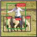
Mission : Locate and classify all objects in the image . This task usually includes : Proposed area , Then classify the objects .
Data sets :PASCAL, COCO
Semantic segmentation (Semantic Segmentation)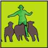
Mission : Mark each pixel of the image with the object class to which the image belongs , For example, the person in this example 、 Sheep and grass .
Data sets : PASCAL, COCO
Instance segmentation (Instance Segmentation)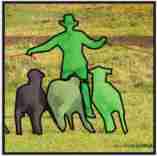
Mission : Mark each pixel of the image with the object class and object instance it belongs to .
Data sets :PASCAL, COCO
Key point detection (Keypoint Detection)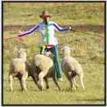
Mission : Detect the position of a set of predefined object keys , Such as key points of human body , Face key points .
Data sets :COCO
Related concepts of convolution network
features (feature)
Pattern (pattern)、 Neurons activate (activation of a neuron)、 Characteristic detector (feature detector) 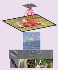
Characteristics refer to : When a particular mode ( features ) Appears in its input field ( Receiving area ) when , Activated hide Neuron
Patterns detected by neurons can be visualized by :
(1) Optimize the input area to maximize the activation of neurons (deep dream)
(2) Visualize the gradient of neuron activation or guiding gradient on the input pixel ( Back propagation and guided back propagation )
(3) Visualize a group of image areas that can most activate neurons in the training data set
Receptive domain (Receptive Field)
Input area of a feature (input region of a feature)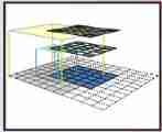
The accepted domain refers to : Input image Areas that affect feature activation . let me put it another way , It is the area concerned by the feature .
Generally speaking , Higher level features have larger acceptance domains , This allows it to learn to capture more complex / Abstract patterns . The structure of convolutional neural network determines how the acceptance domain changes layer by layer .
Characteristics of figure (Feature Map)
A hidden layer channel (a channel of a hidden layer)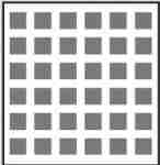
Characteristic diagram refers to : By applying the same Characteristic detector ( filter ) With Sliding window Created by mouth A set of features ( That is convolution )
Features in the same feature map have the same acceptance ability , And look for the same pattern in different places . This produces Space invariance of Convolutional Neural Networks .
Characteristic quantity (Feature Volume)
Hidden layer in convolutional neural network (a channel of a hidden layer)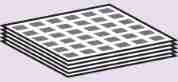
Characteristic quantity refers to A set of feature maps ( Characteristics of figure ), Each feature map searches for features at a fixed position on the input image . All features have the same accepted domain size .
The full connection layer is used as the characteristic quantity (Fully connected layer as Feature Volume)
have k A full connection layer of hidden nodes (fc layer —— Usually connected to the end of convolutional neural network for classification ) Can be seen as a 1x1xk Characteristic quantity of .
This feature quantity has a feature in each feature graph , Its acceptance domain covers the entire image . Will a 1x1xk Filter core with a 1x1xd The characteristic volume of , Will create a 1x1xk Feature volume . Replace completely connected layers with convoluted layers , It enables us to apply convolution networks to images of any size .
Transposition convolution (Transposed Convolution)
The gradient operation of back propagation convolution operation . let me put it another way , It is the backward transmission of convolution . A transposed convolution can be realized as a normal convolution inserting zero between input features . The size of a filter is k, stride s And zero padding p The convolution of has a related transpose convolution , Its filter size is k ’ =k, stride s ’ =1, Zero fill p ’ =k-p-1, And insert s-1 0.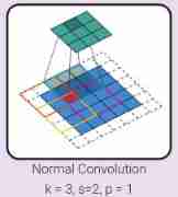
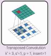
As shown in the picture above on the left , The red input unit helps activate the 4 Output units ( adopt 4 Colored squares ), Therefore, it receives gradients from these output units . This gradient back propagation can be achieved by transpose convolution shown on the right .
End to end object recognition system (End-To-End object recognition pipeline)
By optimizing a single objective function ( That is, the differentiable function of variables in each stage ) To train all stages ( Preprocessing 、 Regional proposal generation 、 Proposal classification 、 post-processing ) Target recognition process This end-to-end system is opposite to the traditional object recognition system , The latter connects the stages in a non differentiable way . In these systems , We don't know how changing the variables of a stage will affect the overall performance , So each stage must be trained independently or alternately , Or heuristic programming .
Related concepts of object detection (Object Recognition Concepts)
The bounding box proposes (Bounding box proposal)
Areas of interest (region of interest), Regional proposal (region proposal), Box proposal (box proposal)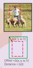
Input a rectangular area in the image that may contain objects . These suggestions can be generated by some heuristic search : Object search 、 Selective search or regional suggestion network (RPN). It can be expressed as a bounding box 4 Unit vector , Or store its two angular coordinates (x0, y0) (x1, y1), or ( More common ) Store its center position and its width and height (x, y, w h). A bounding box is usually accompanied by a confidence score ( That is, judge how likely the detection box contains objects ). The difference between two bounding boxes is usually represented by their vectors L2 Distance to measure .W and h Logarithmic transformation can be carried out before calculating the distance .
Occurring simultaneously than (Intersection over Union、IOU)
Measure the similarity between the real frame and the detection frame 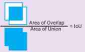
Non maximum suppression (Non Maxium Suppression、NMS)
Any detection frame that significantly overlaps with the detection frame with higher reliability (IoU > IoU_threshold) Be inhibited ( Delete ).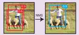
Bounding box regression( Regression of bounding box )
By observing the input area , We can infer the bounding box that is more suitable for the object in it , Even if the object is only partially visible . The above example shows that it can be inferred by observing only a part of the object ground truth box The possibility of .
therefore , A regressor can be trained to observe an input region , Predict the offset between the input field box and the truth box ∆(x, y, w, h). If every object class has a regressor , It is called the regression of specific classes , Otherwise, it is called class independent regression ( All classes have a regressor ).
Bounding box regressors are usually accompanied by a bounding box classifier ( Confidence scorer ) To estimate the confidence that the object exists in the box . Classifiers can also be class specific or class independent . If the front box is not defined , The input area box plays the role of the previous box .
A priori box (Prior box)
Unlike using the input field as the only a priori box , We can train multiple bounding box regressors , Each regressor looks at the same input field , But there are different a priori frames , And learn to predict the offset between your prior box and the ground truth box . such , Regressors with different prior frames can learn to predict different properties ( Aspect ratio 、 The proportion 、 Location ) The bounding box of . The previous box can be predefined relative to the input area , Or learn through clustering . The correct box matching strategy is the key to make the training converge .
Check box matching strategy (Box matching Strategy)
We cannot expect the bounding box regressor to predict the distance from the input region or a priori box ( More common ) Objects too far away . therefore , We need a matching strategy to decide which a priori box matches the real value . Each match is a training example for regression . Possible strategies :( Multiple boxes ) Match each real box with a previous highest IOU A priori box match of ;
Full picture ~
边栏推荐
- 六月刷题01——数组
- Bugku web guide
- Hard core! One configuration center for 8 classes!
- Configure system environment variables through bat script
- 嵌入式開發中的防禦性C語言編程
- C杂讲 双向循环链表
- 六月刷题02——字符串
- Elk project monitoring platform deployment + deployment of detailed use (II)
- MapReduce instance (VI): inverted index
- June brush question 01 - array
猜你喜欢
Learning SCM is of great help to society
O & M, let go of monitoring - let go of yourself
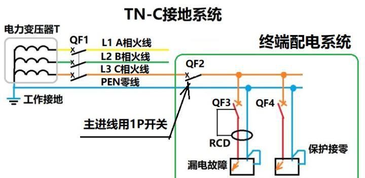
tn-c为何不可用2p断路器?
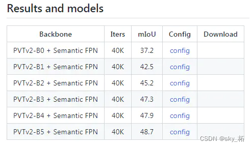
![[deep learning] semantic segmentation: paper reading: (CVPR 2022) mpvit (cnn+transformer): multipath visual transformer for dense prediction](/img/f1/6f22f00843072fa4ad83dc0ef2fad8.png)
[deep learning] semantic segmentation: paper reading: (CVPR 2022) mpvit (cnn+transformer): multipath visual transformer for dense prediction

Some thoughts on the study of 51 single chip microcomputer
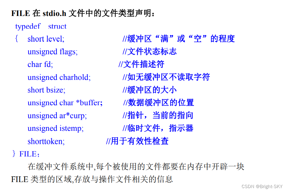
C杂讲 文件 初讲
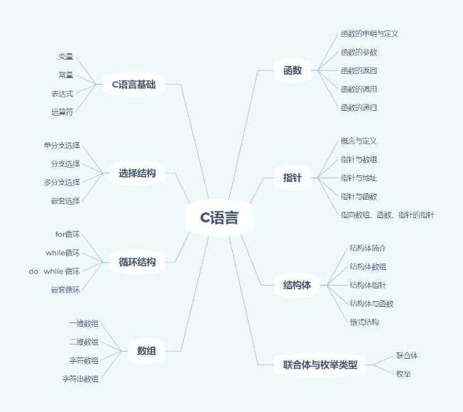
How can I take a shortcut to learn C language in college
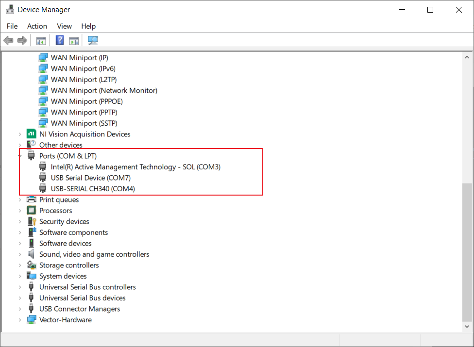
Canoe cannot automatically identify serial port number? Then encapsulate a DLL so that it must work
Segmentation sémantique de l'apprentissage profond - résumé du code source
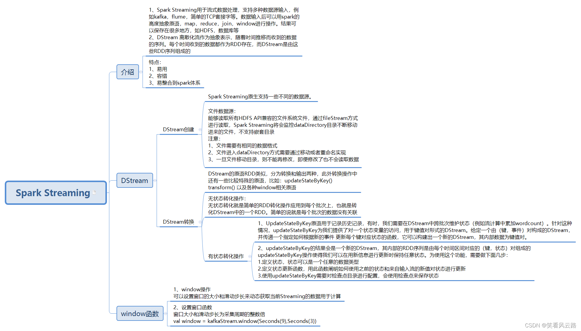
Take you back to spark ecosystem!
随机推荐
MapReduce instance (V): secondary sorting
大学C语言入门到底怎么学才可以走捷径
Why is 51+ assembly in college SCM class? Why not come directly to STM32
Design and implementation of online snack sales system based on b/s (attached: source code paper SQL file)
MapReduce instance (IX): reduce end join
手把手教您怎么编写第一个单片机程序
CANoe的数据回放(Replay Block),还是要结合CAPL脚本才能说的明白
Interview shock 62: what are the precautions for group by?
June brush question 02 - string
June brush question 01 - array
Canoe cannot automatically identify serial port number? Then encapsulate a DLL so that it must work
五月集训总结——来自阿光
Release of the sample chapter of "uncover the secrets of asp.net core 6 framework" [200 pages /5 chapters]
一大波開源小抄來襲
Oom happened. Do you know the reason and how to solve it?
C杂讲 动态链表操作 再讲
在CANoe中通过Panel面板控制Test Module 运行(高级)
Regular expressions are actually very simple
The replay block of canoe still needs to be combined with CAPL script to make it clear
DCDC power ripple test