当前位置:网站首页>HDR image reconstruction from a single exposure using deep CNN reading notes
HDR image reconstruction from a single exposure using deep CNN reading notes
2022-07-06 22:14:00 【Cassia tora】
HDR image reconstruction from a single exposure using deep CNNs Reading notes
The paper was published in 2017 Year of TOG.
1 Abstract
problem :
Low dynamic range (LDR) Device capture high dynamic range (HDR) Scene images are prone to overexposure , Overexposed areas will lose texture details , Bring challenges to image viewing or computer vision tasks .
present situation :
Most of the existing HDR Image reconstruction methods require a set of different exposures LDR Image as input .
Methods of this paper :
It solves the problem of estimating the missing information in the saturated region of the image , In order to be able to From single exposure LDR High quality image reconstruction HDR Images .
(1)LDR The input image is converted by the encoder network , Represented by compact features that generate image spatial context .
(2) The encoded image is fed to HDR Decoder network , To rebuild HDR Images .
The network is equipped with Jump connection , Can be found in LDR Encoder and HDR Transmit data between decoder domains , In order to make full use of high-resolution image details in reconstruction .
2 HDR Reconstruction Model
2.1 Formulation and constraints of the problem (Problem formulation and constraints)
Final HDR Reconstruct pixels H ^ ( i , c ) \hat{H}_{(i,c)} H^(i,c), Is to use mixed values (blend value) α i α_i αi Pixel level blending (blending) Calculated ,
i i i: Spatial index
c c c: Color channel
D ( i , c ) D_{(i,c)} D(i,c): Input LDR Image pixels
y ^ ( i , c ) \hat{y} _{(i,c)} y^(i,c):CNN Output ( In the logarithmic field ):
f ( − 1 ) f^{(-1)} f(−1): Inverse camera curve , Transform the input into a linear field .
blend (blending) It's a linear slope , From threshold τ τ τ Start with the pixel value of , To the end of the maximum pixel value ( Blending means that the input image remains unchanged in the unsaturated region ),
This article USES the τ = 0.95 τ=0.95 τ=0.95, The input is defined in [ 0 , 1 ] [0,1] [0,1] Within the scope of .
Linear mixing (linear blending) It prevents band artifacts between the predicted highlight and its surrounding environment ( α α α It is also used to define the loss function in training , As the first 2.4 Section ).
The description of the mixing component is shown in the figure below ( Since the focus of hybrid prediction is the reconstruction around the saturated region , Therefore, artifacts may appear in other image areas ( chart (b))):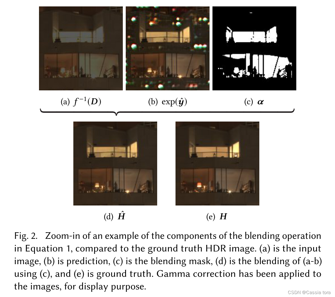
2.2 Hybrid dynamic range automatic encoder (Hybrid dynamic range autoencoder)
The complete automatic encoder architecture is shown in the figure :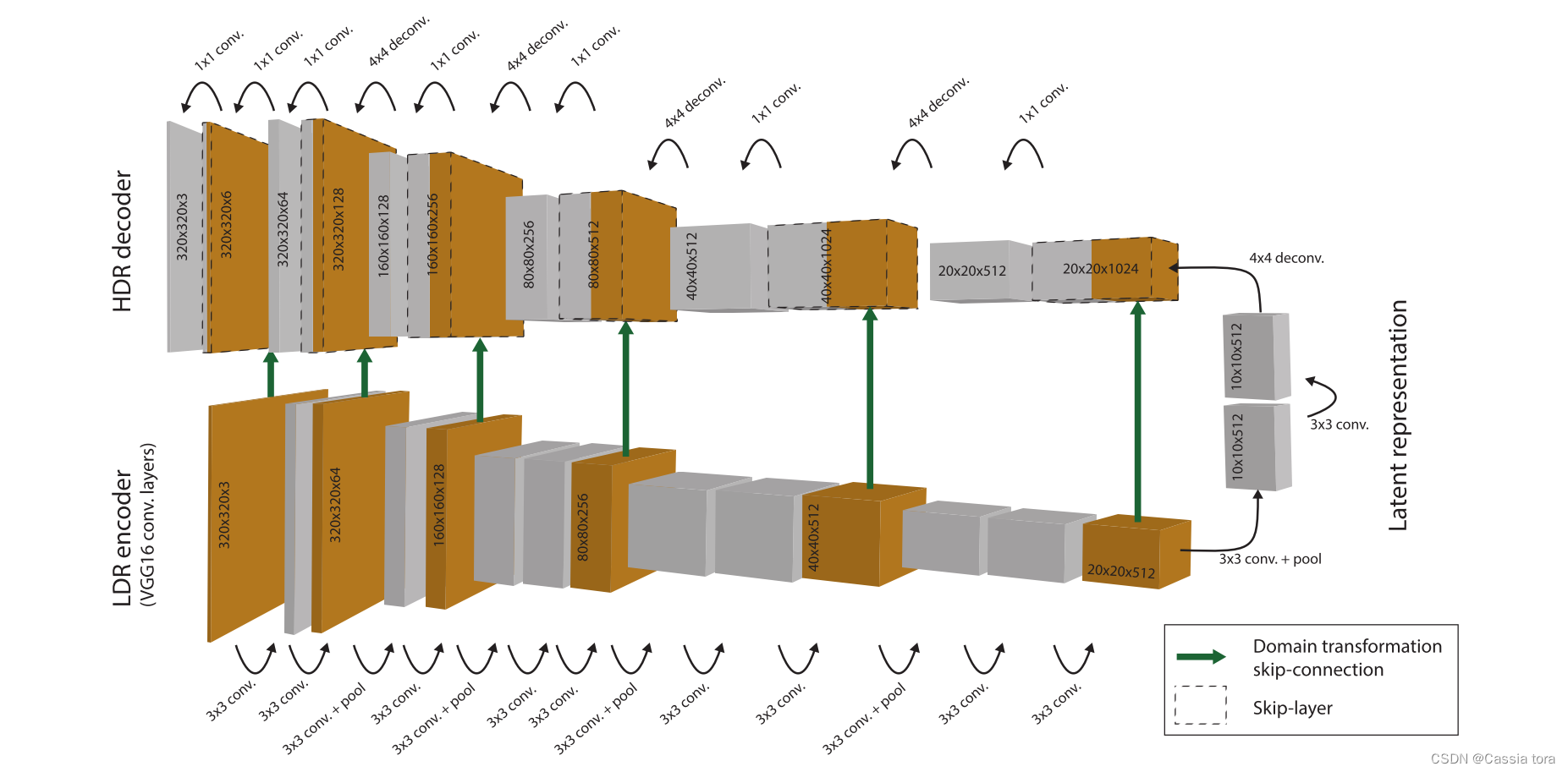
LDR encoder: For the input LDR Image convolution and maximum pooling , The resulting W / 32 × H / 32 × 512 W/32 ×H/32 ×512 W/32×H/32×512 The low dimensional latent image of (latent image representation)( W W W and H H H Image width and height ).
HDR decoder: Use 4 × 4 4×4 4×4 Deconvolution of Realize bilinear up sampling , Jump and connect the result of up sampling with the corresponding layer of the encoder ( Better restore image details ), Convolute the jump connection results ; Repeat the above operation , Finally rebuild the high dimension HDR Images .
(1) Because the goal of this paper is to reconstruct a larger image than the image actually used in training , So the potential means Not a fully connected layer , It is Low resolution multi-channel image . This full convolution network (FCN) It can be predicted at any resolution , The resolution is a multiple of the reduction factor of the automatic encoder .
(2) Because the encoder is directly on LDR Input image for operation , The decoder is responsible for generating HDR data , therefore The decoder works in the log domain ( This is achieved by using the loss function , This function compares the network output with HDR gt Compare the logarithm of the image ).
(3) All layers of the network Use ReLU Activation function , After each layer of the decoder Use batch normalization layer .
2.3 Domain transformation and jump connection (Domain transformation and skip-connections)
The layer by layer convolution pooling of input images will lead to the loss of many high-resolution information of early layers , The decoder can use this information to reconstruct the high-frequency details of the saturated region , Therefore, jump connection is introduced , Used to transmit data between high-level and low-level features in encoder and decoder .
The automatic encoder in this paper uses hopping connection to transmit each layer of the encoder to the corresponding layer of the decoder . Because the encoder and decoder process different types of data ( See the first 2.2 section ), Connections include domain transformations and logarithmic transformations described by inverse camera curves , take LDR The display value maps to logarithm HDR Express . This article uses gamma function f − 1 ( x ) = x γ f^{-1} (x)=x^γ f−1(x)=xγ To complete the linearization of jump connection , among γ = 2 γ=2 γ=2.
This paper connects two layers along the feature dimension , That is the two one. W × H × K W×H×K W×H×K Dimension layer connection is W × H × 2 K W×H×2K W×H×2K layer . Then the decoder linearly combines these features , Equivalent to passing 1 × 1 1×1 1×1 The convolution layer of will 2 K 2K 2K The number of features is reduced to K K K. complete LDR To HDR Jump connection is defined as :
h i E , h i D h_i^E,h_i^D hiE,hiD: Encoder layer and decoder layer tensors y E , y D ∈ R ( W × H × K ) y^E,y^D∈R^(W×H×K) yE,yD∈R(W×H×K) All characteristic channels of k ∈ 1 , . . . , K k∈{1,...,K} k∈1,...,K Slice on
h ~ i D \tilde{h} _i^D h~iD: Decoder eigenvector , It has a connection vector from jump h i E h_i^E hiE Fused information
b b b: Deviation of feature fusion
σ σ σ: Activation function , This article USES the ReLU function
( Use small constants in domain transformations ϵ ϵ ϵ To avoid zero in logarithmic transformation .)
Given K K K Features , h E and h D h^E and h^D hE and hD yes 1 × K 1×K 1×K Vector , W W W It's a 2 K × K 2K×K 2K×K The weight matrix of , It will 2 K 2K 2K The features in series are mapped to K K K dimension . It is initialized to perform the addition of encoder and decoder features , Set the weight to 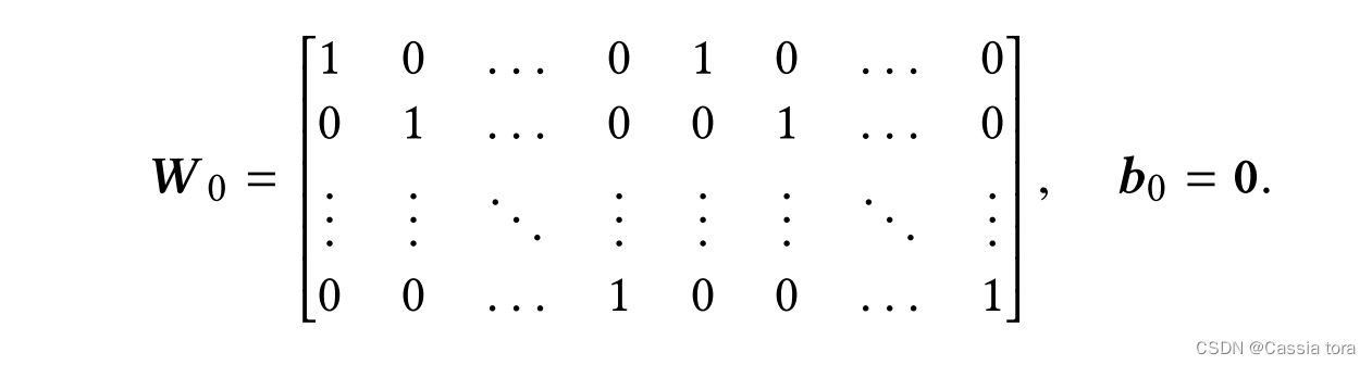
Adding jump connections can better reconstruct image texture details , As shown in the figure :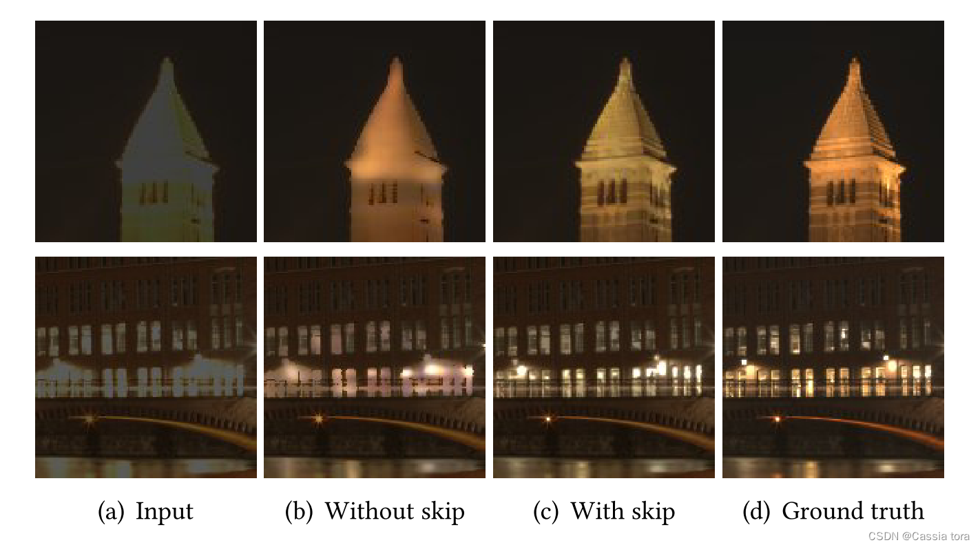
2.4 HDR Loss function (HDR loss function)
Direct loss L ( y ^ , H ) L(\hat{y},H) L(y^,H):
In this system ,HDR The decoder is designed to run in the log domain . therefore , In the logarithm of a given prediction HDR Images y ^ \hat{y} y^ And linear gt Images H Under the circumstances , Direct loss in logarithm HDR The value is formulated ,
N N N: sizes
H ( i , c ) H_{(i,c)} H(i,c): H ( i , c ) ∈ R + H_{(i,c)}∈\mathbb{R}^+ H(i,c)∈R+
ϵ ϵ ϵ: Small constant , Eliminate singularity at zero pixel value
Weber-Fechner The law implies Logarithmic relationship between physical brightness and perceived brightness , Therefore, the loss formulated in the logarithmic domain makes the perception error roughly evenly distributed over the entire brightness range .
I/R Loss L I R ( y ^ , H ) L_{IR}(\hat{y} ,H) LIR(y^,H):
It is meaningful to deal with the illuminance and reflectance components separately , Therefore, this paper proposes another loss function , Deal with illumination and reflectivity respectively . Lighting component I I I Describe global changes , And responsible for high dynamic range ; Reflectivity R R R Store information about details and colors , This has a low dynamic range , H ( i , c ) = I i R ( i , c ) H_{(i,c)}=I_iR_{(i,c)} H(i,c)=IiR(i,c). Through logarithmic brightness L y ^ L^{\hat{y}} Ly^ Gaussian low pass filter G σ G_σ Gσ To approximate logarithmic illuminance , Through the logarithm of prediction HDR Images y ^ \hat{y} y^ And logarithmic illuminance to approximate logarithmic reflectance ,
L y ^ L^{\hat{y}} Ly^: Linear combination of color channels , L i y ^ = l o g ( ∑ c w c e x p ( y ^ i , c ) ) L^{\hat{y}}_i=log(∑_cw_c exp(\hat{y}_{i,c} ) ) Liy^=log(∑cwcexp(y^i,c)), among w = { 0.213 , 0.715 , 0.072 } w=\{0.213,0.715,0.072\} w={ 0.213,0.715,0.072}.
The standard deviation of Gaussian filter is set to σ = 2 σ=2 σ=2.
Use I I I and R R R The resulting loss function is defined as :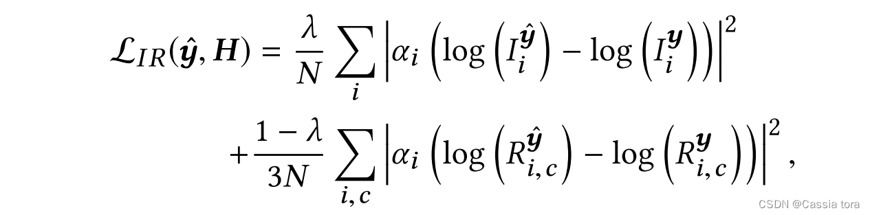
y y y: y = l o g ( H + ϵ ) y=log(H+ϵ) y=log(H+ϵ)
λ λ λ: Equilibrium parameters , Importance of balancing illumination and reflectivity .
This article USES the λ = 0.5 λ=0.5 λ=0.5.
Use different λ λ λ The prediction example results of value optimization are shown in the figure :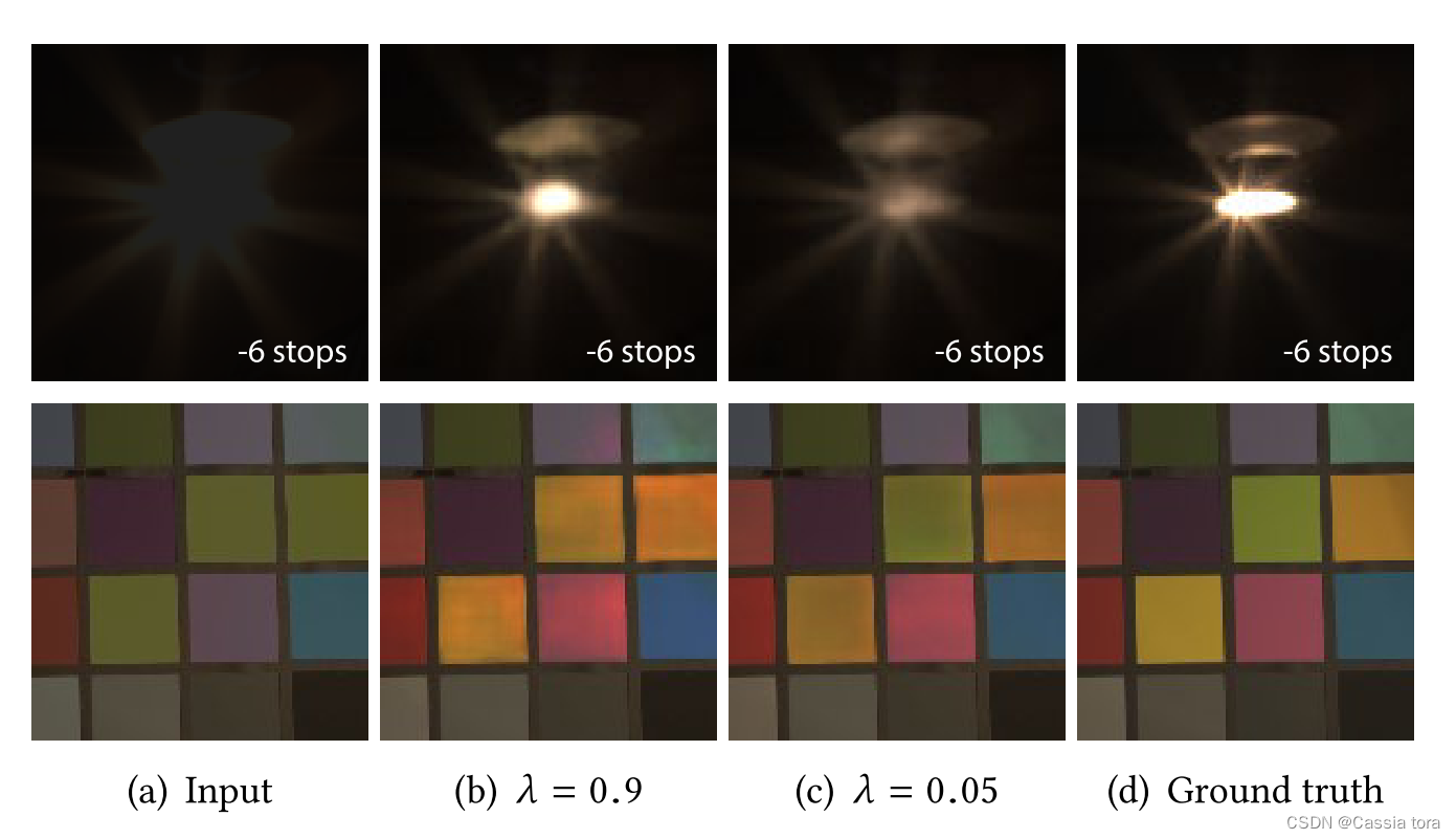
Use I/R Loss , In a large saturated region , It tends to produce less artifacts , As shown in the figure ( One possible explanation is , Gaussian low-pass filter in loss function may have regularization effect , Because it makes the loss in the pixel affected by its neighborhood ):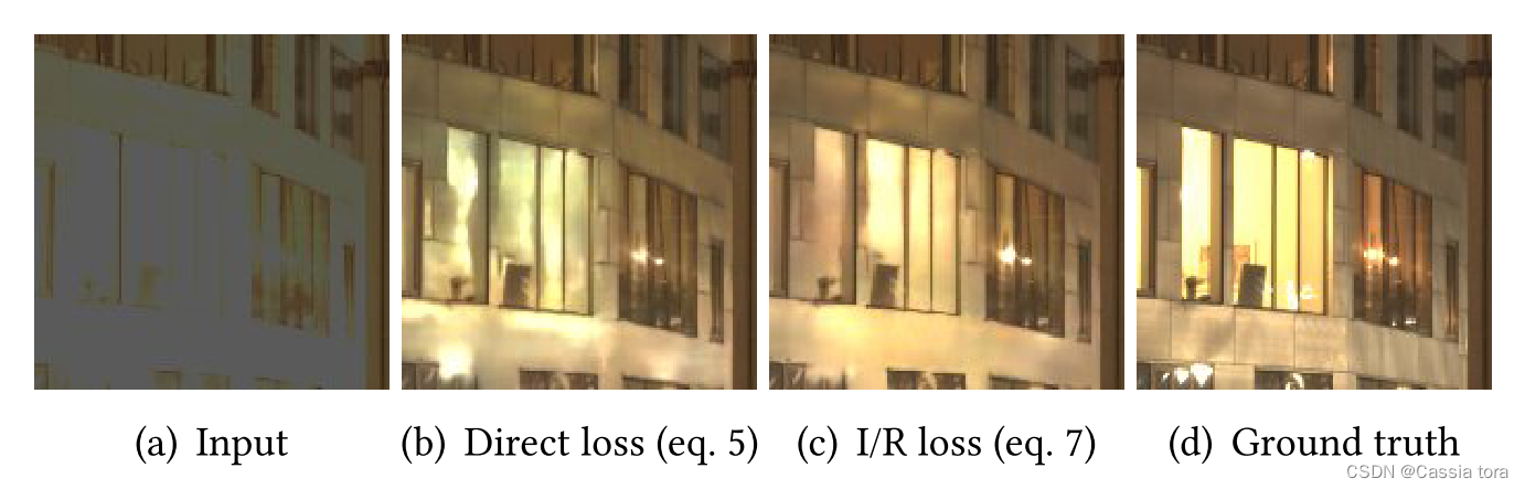
3 HDR Image Dataset
The following figure shows two typical LDR Data sets and 125K Graphic HDR Average histogram of data set .LDR The data are about 2.5M and 200K Of Places and Flickr Image composition ,HDR The data is obtained from HDR Captured in the data set .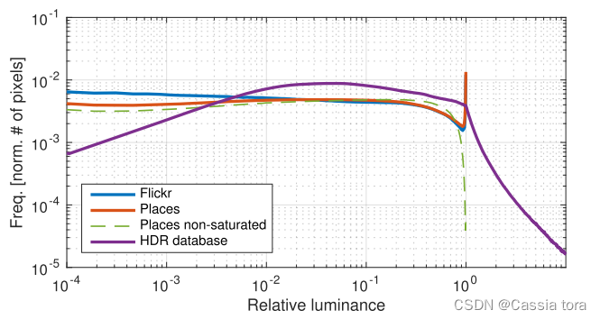
LDR The histogram shows a relatively uniform distribution of pixel values , Except for the obvious peak close to the maximum , Indicates information lost due to saturation .HDR In the histogram , Pixels are not saturated , It is represented by the long tail of exponential decay .
Virtual camera :
Use randomly selected camera calibration to capture multiple random areas of the scene . These areas are selected as image cropping with random size and location , Then flip randomly and resample to 320×320 Pixels . Camera calibration includes exposure 、 Camera curve 、 Parameters such as white balance and noise level . This provides an expanded set of LDR And corresponding HDR Images , Used as training input and gt value .
4 Training
Initialize weights in the network , This paper uses different strategies for different parts of the network .
(1) Due to the use from VGG16 Convolution layer of network , So you can Places The pre training weights that can be used for large-scale image classification are used in the database to initialize the encoder .
(2) Use the decoder to deconvolute for bilinear up sampling , And use the fusion of jump connection layers to perform feature addition .
(3) For potential image representation ( The right side of the network structure diagram ) And final feature reduction ( The upper left corner of the network structure diagram ) Convolution in , This article USES the Xavier initialization .
(4) Use Adam Optimizer on I/R Minimize the loss function , The learning rate is 5 × 1 0 − 5 5×10^{−5} 5×10⁻⁵. In all 800K Step back propagation , Batch size is 8, stay NVIDIA Titan X GPU It takes about 6 God .
4.1 simulation HDR Data pre training (Pre-training on simulated HDR data)
Because of the existing HDR Limited data , The author of this paper through large-scale simulation HDR The entire network is pre trained on the dataset to use migration learning . This article chooses Places Subset of images in the database , It is required that the image should not contain saturated image areas . Give all Places Collection of images P, This subset S ⊂ P \mathbb{S}⊂\mathbb{P} S⊂P Is defined as 
p D p_D pD: Image histogram
ξ ξ ξ: This article USES the ξ = 50 / 25 6 2 ξ=50/256^2 ξ=50/2562( That is, if it is less than 50 Pixel ( Images 25 6 2 256^2 2562 A pixel 0.076%) Has a maximum value of , Then use the image in the training set ).
The green dotted line in the figure below can be seen by comparing with the orange implementation , A subset of S \mathbb{S} S The average histogram on does not show the original set P \mathbb{P} P Saturated pixel peak :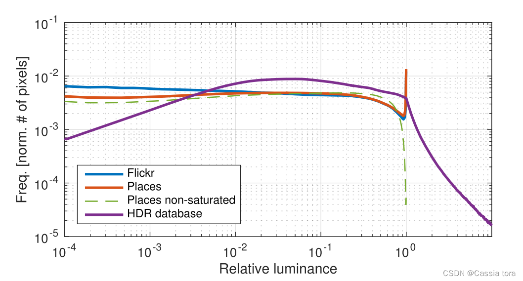
By placing the image D ∈ S D∈\mathbb{S} D∈S Conduct H = s f − 1 ( D ) H=sf^{-1} (D) H=sf−1(D) Linearize and increase exposure , Create a simulation HDR Training data set .
simulation HDR The data set is prepared in the same way as the 3 Same as in section , But the resolution is 224×224 Pixels , No need to resample .CNN Use ADAM The optimizer trains , The learning rate is 2 × 1 0 − 5 2×10^{-5} 2×10⁻⁵, common perform 3.2M Step , Batch is 4.
This pre training of synthetic data results in a significant improvement in performance . As shown in the figure below , Sometimes underestimated small highlights can be better restored , And less artifacts are introduced in the larger saturated region :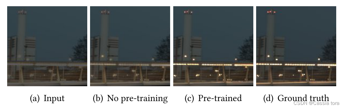
5 Result
5.1 Test error (Test errors)
The following table shows the influence of different training strategies on different errors :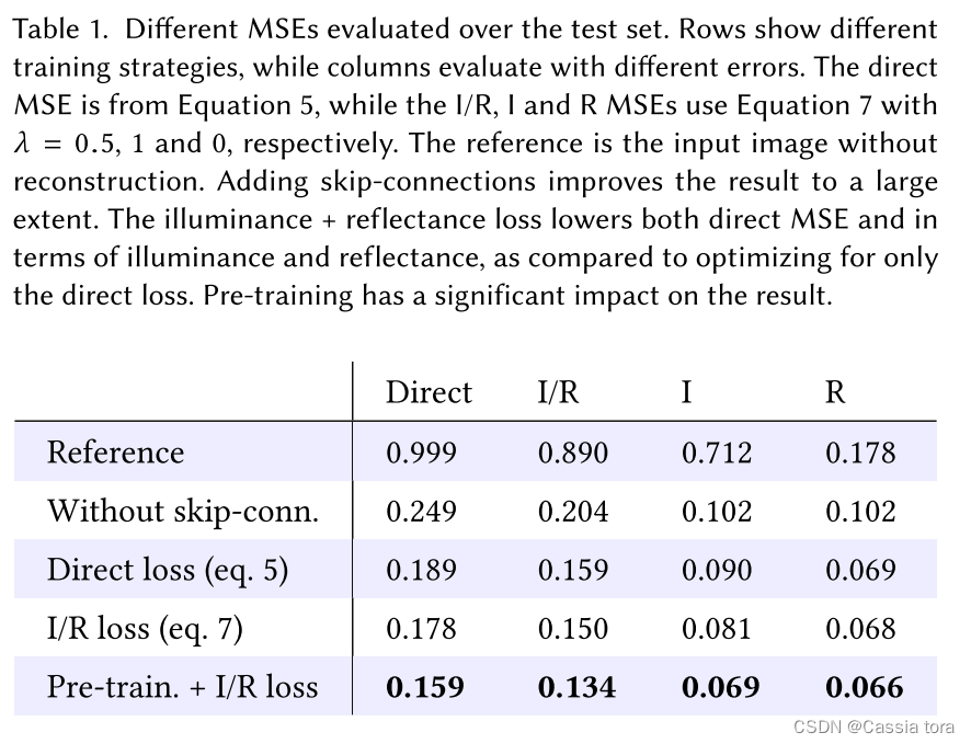
(1) No jump connection CNN It can significantly reduce the input MSE, But adding jump connections can reduce the error 24%, And create images with significantly improved details .
(2) Compare Direct loss and I/R loss,I/R loss stay I/R and Direct MSE Aspect shows low error , Less 5.8%.
(3) Through pre training and I/R loss, Achieve the best training performance , Compared with no pre training , The error is reduced 10.7%.
5.2 And groung truth Compare (Comparisons to ground truth)
The following figure shows the image reconstruction and ground truth Comparison , among input Yes, it will HDR The image is converted by virtual camera LDR Images .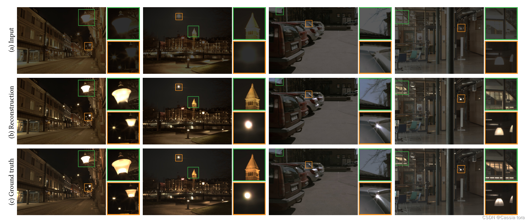
For visualization CNN Reconstructed information , The following figure shows the learning residuals of the image r ^ = m a x ( 0 , H ^ − 1 ) \hat{r}=max(0,\hat{H}-1) r^=max(0,H^−1)( Top left ), as well as ground truth residual r = m a x ( 0 , H − 1 ) r=max(0,H-1) r=max(0,H−1)( The upper right ). The prediction of complex lighting areas is convincing ( The lower left ), But for a very strong spotlight , The brightness is underestimated ( The lower right ).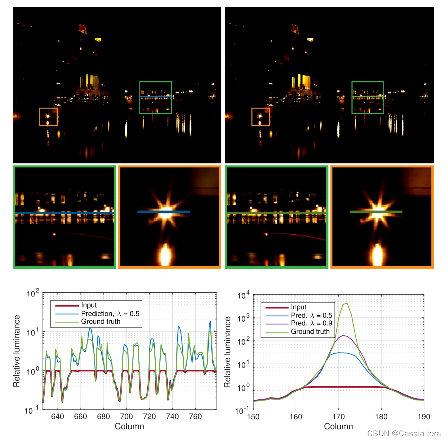
5.3 Reconstruction of real camera images (Reconstruction with real-world cameras)
Use the... Of this article HDR Reconstruct the model to deal with the real camera LDR Images , The results are shown in the following figure :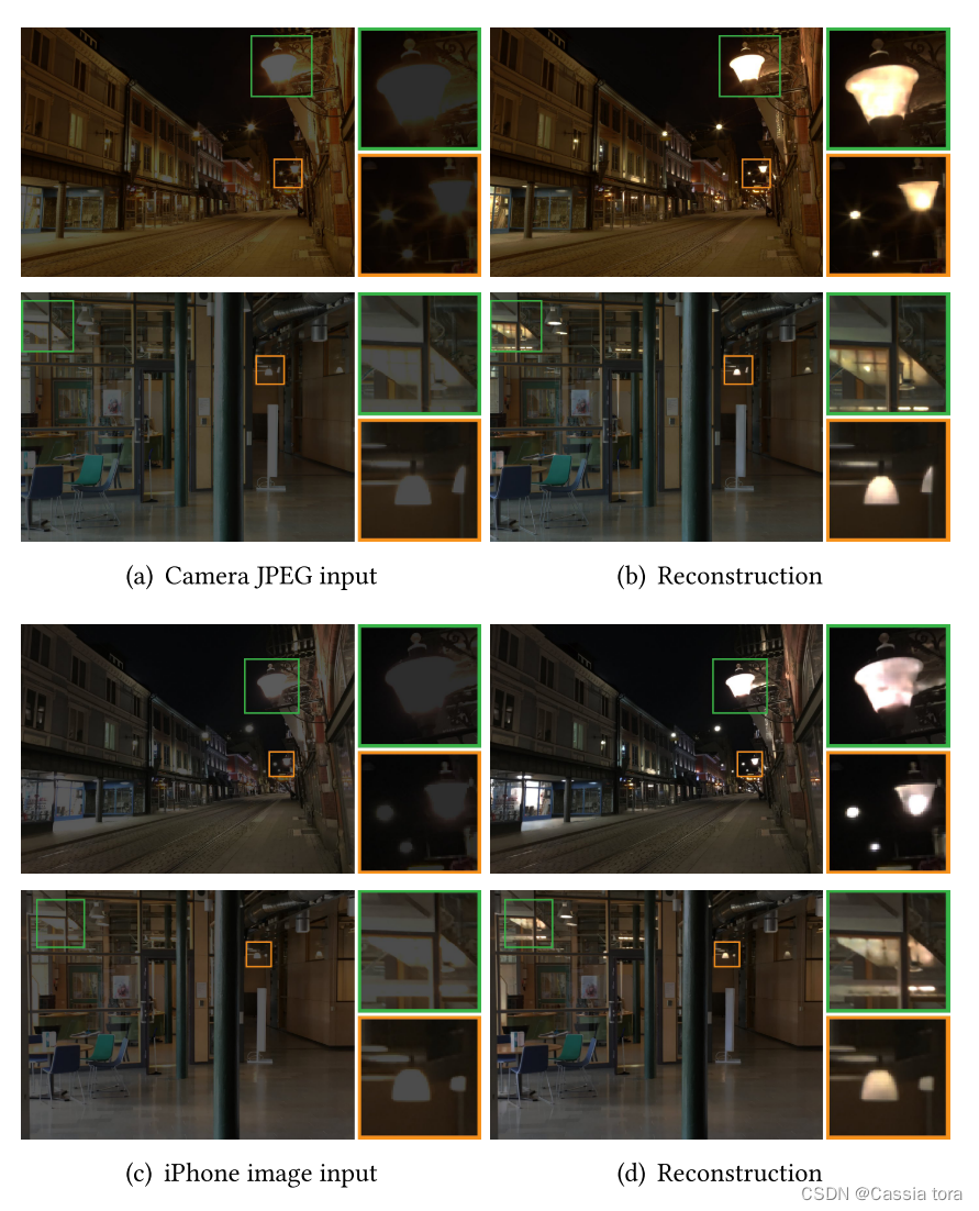
In order to further explore the possibility of reconstructing daily images , The following figure shows a group of pictures taken in various situations iPhone Images :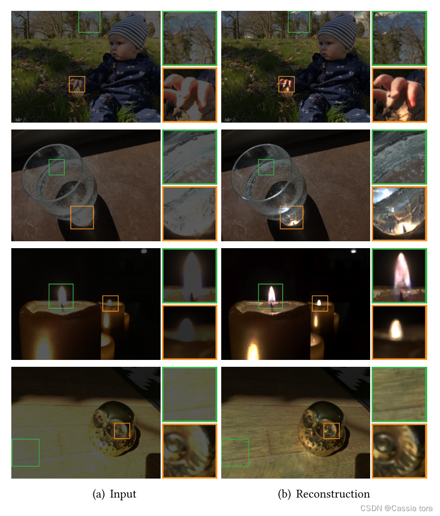
5.4 Change the cut point (Changing clipping point)
The following figure shows the prediction of exposure time of different virtual cameras ( The figure below shows the proportion of pixels in the saturated area in the image , Zoom the image , Make the image have the same exposure after cutting ), It can be seen that more details can be obtained in the reconstruction of shorter exposure images .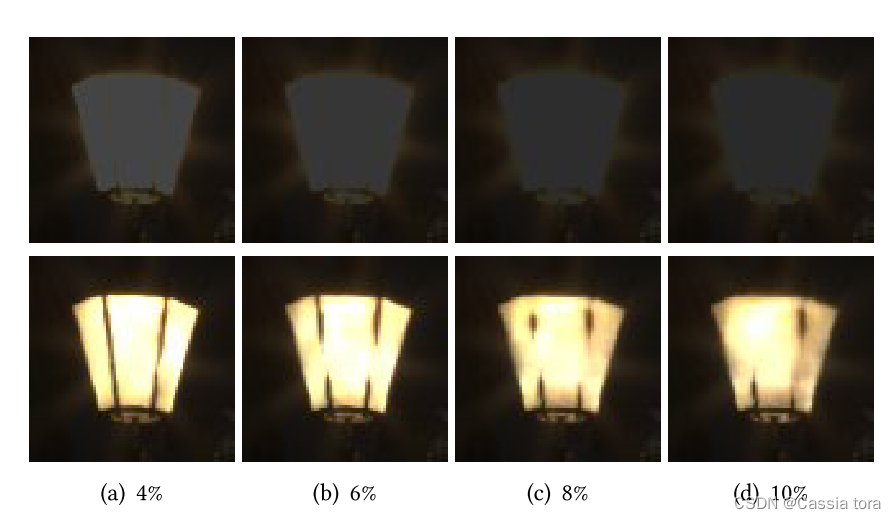
5.5 And iTMOs Compare (Comparison to iTMOs)
this paper HDR The comparison between reconstruction and three existing inverse tone mapping methods is shown in the following figure :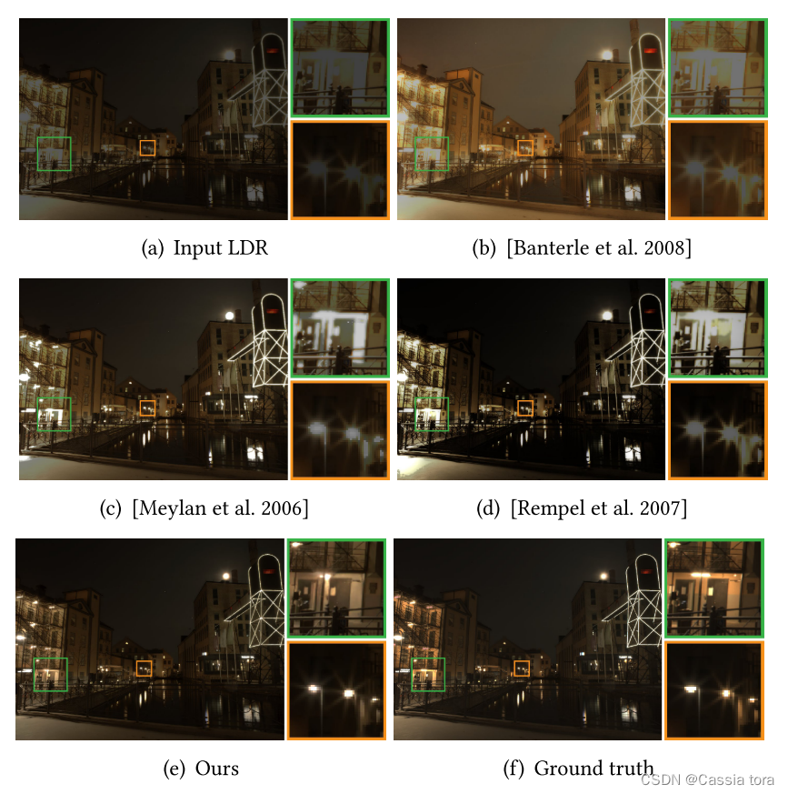
6 Discuss
6.1 Limit
The following figure shows an example of a difficult scenario that this method is difficult to reconstruct :
(1) The first line has a large area with saturation in all color channels , Therefore, it is impossible to infer the structure and details .
(2) The second line shows when an area in the image has extreme intensity , This method will underestimate this extreme intensity .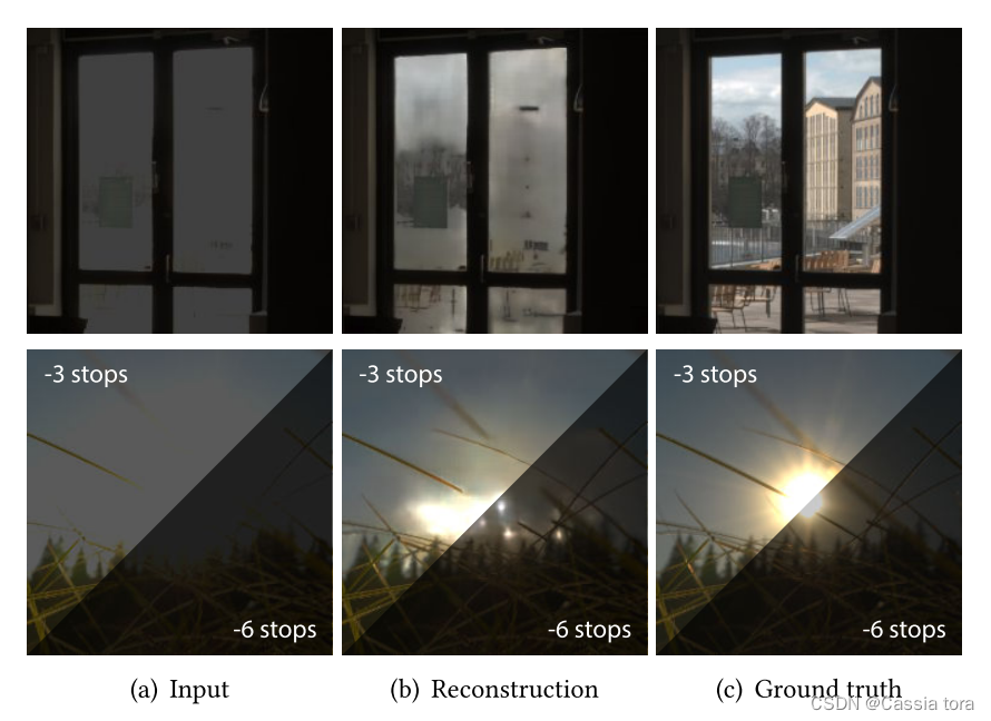
边栏推荐
- Hardware development notes (10): basic process of hardware development, making a USB to RS232 module (9): create ch340g/max232 package library sop-16 and associate principle primitive devices
- 2021 geometry deep learning master Michael Bronstein long article analysis
- 【MySQL】Online DDL详解
- AI 企业多云存储架构实践 | 深势科技分享
- 微信红包封面小程序源码-后台独立版-带测评积分功能源码
- GPS从入门到放弃(十二)、 多普勒定速
- Write a rotation verification code annotation gadget with aardio
- Some problems about the use of char[] array assignment through scanf..
- GPS从入门到放弃(十三)、接收机自主完好性监测(RAIM)
- HDR image reconstruction from a single exposure using deep CNNs阅读札记
猜你喜欢
Earned value management EVM detailed explanation and application, example explanation

墨西哥一架飞往美国的客机起飞后遭雷击 随后安全返航
Management background --3, modify classification
Yyds dry goods inventory C language recursive implementation of Hanoi Tower
ZABBIX proxy server and ZABBIX SNMP monitoring

GNN,请你的网络层数再深一点~
Classic sql50 questions
GPS從入門到放弃(十三)、接收機自主完好性監測(RAIM)
Reset Mikrotik Routeros using netinstall
Powerful domestic API management tool
随机推荐
11、 Service introduction and port
Is it important to build the SEO foundation of the new website
Qt | UDP广播通信、简单使用案例
第3章:类的加载过程(类的生命周期)详解
[Chongqing Guangdong education] Tianjin urban construction university concrete structure design principle a reference
二叉(搜索)树的最近公共祖先 ●●
Record the process of cleaning up mining viruses
Support multiple API versions in flask
Codeforces Round #274 (Div. 2) –A Expression
【sciter】: 基于 sciter 封装通知栏组件
Leetcode learning records (starting from the novice village, you can't kill out of the novice Village) ---1
hdu 4912 Paths on the tree(lca+馋)
GPS from getting started to giving up (16), satellite clock error and satellite ephemeris error
Force buckle 575 Divide candy
BarcodeX(ActiveX打印控件) v5.3.0.80 免费版使用
Management background --3, modify classification
GNN,请你的网络层数再深一点~
Leveldb source code analysis series - main process
基于LM317的可调直流电源
【10点公开课】:视频质量评价基础与实践