当前位置:网站首页>Introduction to deep learning Ann neural network parameter optimization problem (SGD, momentum, adagrad, rmsprop, Adam)
Introduction to deep learning Ann neural network parameter optimization problem (SGD, momentum, adagrad, rmsprop, Adam)
2022-07-04 06:57:00 【Mud stick】
Here's the catalog title
1. Parameter optimization
This article summarizes ANN Various methods of parameter update
Some mathematical formulas that may be used The mathematical formula
1.1 Random gradient descent method (SGD)
We used the random gradient descent method in the previous chapter (SGD) Update parameters , Here it is , We will propose other methods to optimize parameters , And point out that SGD Some shortcomings of .
Let's understand the process of finding the optimal parameters through a story :
Under such harsh conditions , Ground slope is particularly important , Feel the inclination of the ground through the soles of your feet , Namely SGD The strategy of . brave Explorers may think that just repeat this strategy , One day we can reach “ The deepest place ”.
1.1.2SGD
The random gradient descent method can be written as the following formula
![[ Failed to transfer the external chain picture , The origin station may have anti-theft chain mechanism , It is suggested to save the pictures and upload them directly (img-hkbLC8GG-1644804304270)( 6、 ... and 、 Skills related to neural network learning .assets/ chart 6-2.png)]](/img/10/0b4a1e7012f3525e3cdbcd6da0bb7e.jpg)
Let's implement a program named SGD Class
class SGD:
	def __init__(self, lr=0.01):
 		self.lr = lr

 	def update(self, params, grads):
 		for key in params.keys():
 		params[key] -= self.lr * grads[key]
If you have studied the previous chapters , This code is easy to understand .
update Functions are constantly called to update parameters .
We can train neural networks as follows ( Pseudo code , Can not run )
network = TwoLayerNet(...)
optimizer = SGD()
for i in range(10000):
	...
 	x_batch, t_batch = get_mini_batch(...) # mini-batch
 	grads = network.gradient(x_batch, t_batch)
 	params = network.params
 	optimizer.update(params, grads)
here optimizer Express “ People who optimize ” It means , It is responsible for updating parameters .
such , Function modules will become very simple .
1.1.3 SGD The shortcomings of
SGD It's simple and easy to implement , But it may not be efficient in solving some problems , Let's give you an example , Find the minimum value of the following function .
![[ Failed to transfer the external chain picture , The origin station may have anti-theft chain mechanism , It is suggested to save the pictures and upload them directly (img-R1Vm5H21-1644804304271)( 6、 ... and 、 Skills related to neural network learning .assets/ chart 6-3.png)]](/img/0a/29a8b439884aaeee00603c4a56a0fa.jpg)
We can go through matplotlib Let's take a look at this function . The code is as follows
import matplotlib.pyplot as plt
import numpy as np
from mpl_toolkits.mplot3d import axes3d

def f(x,y):
    return 0.05*(x**2)+y**2


# Wireframe
fig = plt.figure()
ax = plt.axes(projection='3d')
#X = np.linspace(-10,10,256)
#Y = np.linspace(-10,10,256)
X = np.linspace(-10,10)
Y = np.linspace(-10,10)
print(f(0,0))
X, Y = np.meshgrid(X, Y)# Generate grid point coordinate matrix .
Z = f(X,Y)
plt.xlabel("x")
plt.ylabel("y")
ax.set_zlabel("z")

ax.plot_wireframe(X, Y, Z, color='black')
ax.set_title('wireframe')
# Contour map
fig2 = plt.figure()
level = np.array([0.0,1,2,3])
C = plt.contour(X, Y, Z,levels=level)
plt.clabel(C,inline=True,fontsize=10)
plt.contour(X,Y,Z)
plt.xlabel("x")
plt.ylabel("y")


plt.show()
![[ Failed to transfer the external chain picture , The origin station may have anti-theft chain mechanism , It is suggested to save the pictures and upload them directly (img-Lc7WeMvl-1644804304271)( 6、 ... and 、 Skills related to neural network learning .assets/ chart 6-4-1644548801104.png)]](/img/17/fc4243fa9220317dd51a483314ec55.jpg)
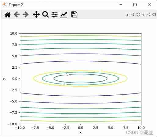
It is not difficult to see from the two pictures ,Z The value of x and y All to 0 Point down , however y The gradient of descent is larger .
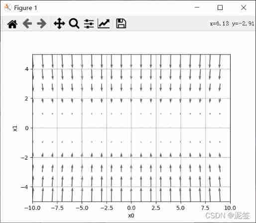
Next, let's use a graph to show the gradient . The code is as follows , The function of finding gradient is familiar to you in the previous chapter
import numpy as np
import matplotlib.pyplot as plt
from deeplearning.fuction import numerical_gradient


def f(x):
    return np.sum(0.05*x[0]**2+x[1]**2)

x = np.arange(-10,10)
y = np.arange(-5,6)
X,Y = np.meshgrid(x,y)
X = X.flatten()
Y = Y.flatten()
a = np.array([X, Y])
grad = numerical_gradient(f,a)

plt.figure()
plt.quiver(X, Y, -grad[0], -grad[1], angles="xy", color="#666666")  # ,headwidth=10,scale=40,color="#444444")
plt.xlim([-10, 10])
plt.ylim([-5, 5])
plt.xlabel('x0')
plt.ylabel('x1')
plt.grid()

plt.draw()
plt.show()
that , Next we use SGD To update the parameters , First, implement SGD Of optimizer.
class SGD:
    def __init__(self,lr = 0.01):
        self.lr = lr

    def update(self,params,grads):
        for key in params.keys():
            params[key]-=self.lr * grads[key]
import numpy as np
import matplotlib.pyplot as plt
from optimizer import SGD

def f(x, y):
    return x**2 / 20.0 + y**2


def df(x, y): # Write the derivative function directly , Omit the gradient
    return x / 10.0, 2.0*y

init_pos = (-7.0, 2.0)
params = {
    }
params['x'], params['y'] = init_pos[0], init_pos[1]
grads = {
    }
grads['x'], grads['y'] = 0, 0

x_history = []
y_history = []

optimizer = SGD(0.95)
for i in range(30):
    x_history.append(params['x'])
    y_history.append(params['y'])

    grads['x'], grads['y'] = df(params['x'], params['y'])
    optimizer.update(params,grads)


for i in range(len(x_history)):
    print(x_history[i],y_history[i])

x = np.arange(-10,10,0.01)
y = np.arange(-5, 5, 0.01)
X,Y = np.meshgrid(x,y)
Z = f(X,Y)


mask = Z > 7
Z[mask] = 0


plt.plot(x_history, y_history, 'o-', color="red")
plt.contour(X, Y, Z)

plt.ylim(-10, 10)
plt.xlim(-10, 10)
plt.plot(0, 0, '+')

plt.xlabel("x")
plt.ylabel("y")
plt.title("SGD")

plt.show()
![[ Failed to transfer the external chain picture , The origin station may have anti-theft chain mechanism , It is suggested to save the pictures and upload them directly (img-w12xUh4N-1644804304272)( 6、 ... and 、 Skills related to neural network learning .assets/ chart 6-7-1644719417221.png)]](/img/16/353a1744bcf1cdde0a1ab0786148d0.jpg)
In the picture ,SGD a “ And ” Glyph movement . This is a rather inefficient path . in other words , SGD The disadvantage of , If the shape of the function is non-uniform (anisotropic), For example, it is extended , Search for The path will be very inefficient . There is a loop print in the middle of this code , Let's look directly at the printed data .
-7.0 2.0
-6.335 -1.7999999999999998
-5.733175 1.6199999999999997
-5.188523375 -1.4579999999999997
-4.695613654375 1.3121999999999998
-4.249530357209375 -1.18098
-3.8458249732744845 1.0628819999999997
-3.4804716008134085 -0.9565937999999994
-3.1498267987361346 0.8609344199999993
-2.8505932528562017 -0.7748409779999994
-2.5797868938348625 0.6973568801999994
-2.3347071389205505 -0.6276211921799995
-2.112909960723098 0.5648590729619996
-1.9121835144544037 -0.5083731656657995
-1.7305260805812355 0.4575358490992195
-1.566126102926018 -0.41178226418929753
-1.4173441231480464 0.37060403777036777
-1.282696431448982 -0.333543633993331
-1.1608402704613288 0.3001892705939978
-1.0505604447675025 -0.270170343534598
-0.9507572025145898 0.2431533091811382
-0.8604352682757038 -0.21883797826302437
-0.778693917789512 0.19695418043672192
-0.7047179955995084 -0.17725876239304972
-0.6377697860175552 0.15953288615374472
-0.5771816563458875 -0.14357959753837024
-0.5223493989930281 0.12922163778453322
-0.4727262060886904 -0.11629947400607987
-0.42781721651026483 0.10466952660547188
-0.3871745809417897 -0.09420257394492468
Process finished with exit code 0
It's easy to see y Although the value of is approaching 0 But it jumps repeatedly between positive and negative ,x The value of is slowly approaching 0.
In the vertical direction , The gradient is very large , In the horizontal direction , The gradient is relatively small , So when we set the learning rate, we can't set it too large , In order to prevent parameter updating in the vertical direction, too much , Such a small learning rate leads to too slow updating of parameters in the horizontal direction , So it leads to very slow convergence .
therefore , We need more than just moving in a gradient SGD More intelligent A clear way .SGD The root cause of inefficiency is , The direction of the gradient does not point in the direction of the minimum .
1.2 Momentum Momentum method
Momentum yes “ momentum ” It means , It's about physics . The mathematical formula is as follows
![[ Failed to transfer the external chain picture , The origin station may have anti-theft chain mechanism , It is suggested to save the pictures and upload them directly (img-Ko6Hb1Q7-1644804304272)( 6、 ... and 、 Skills related to neural network learning .assets/ chart 6-8.png)]](/img/5c/52815d50a043163fe0ef37dd03bf77.jpg)
New variable v Corresponding to the physical speed . It's like a ball rolling on the ground
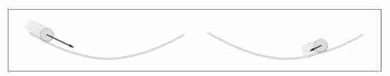
You can think about it , The ball will be faster and faster before it reaches the lowest point , After the lowest point , The speed will rise more and more slowly , Then the speed drops faster and faster , Repeat this process until it stops at the lowest point .
Analyze the above formula ,α Is a momentum parameter , We usually set it to be less than 1 Positive number of , for example 0.9.v Is the parameter added in the last update . We are familiar with others
for instance , If the above ball is at the lowest point x The value is 0, Left x The value is negative. , To the right x The value is positive . Initial value ,x The value is -3,v by 0, Learning rate * gradient =-1,( hypothesis α=0.9).
Update parameters for the first time ,v=0.9 * 0-(-1)=1,x = x+1=-2.
Update parameters for the second time , Suppose the rate of learning * The gradient is still -1:v =0.9 * 1-(-1)= 1.9,x=x+v=-0.1
Update parameters for the third time , Suppose the rate of learning * The gradient is still -1:v=0.9 * 1.9 = 1.71,x=x+v = 1.61
Update parameters for the fourth time ,( In the opposite direction ) Learning rate * gradient =1:v = 0.9 *1.71 - 1=0.539,x = x+v=3.149
We can clearly see , If the direction does not change ,v The value of will gradually increase , That is, the update range will be larger and larger , If the direction changes ,v The value of becomes smaller , The update range will be smaller . It is equivalent to every time when updating parameters , Will take into account the previous speed , The moving range of each parameter in each direction depends not only on the current gradient , It also depends on whether the gradients in the past are consistent in all directions , If a gradient keeps updating along the current direction , Then the range of each update will be larger and larger , If a gradient changes constantly in one direction , Then its update amplitude will be attenuated , In this way, we can use a larger learning rate , Make convergence faster , At the same time, the direction with larger gradient will reduce the amplitude of each update due to momentum .( This paragraph is quoted from here , I think it's very clear )
Now let's talk about the code :
class Momentum:
    def __init__(self,lr = 0.01,momentum = 0.9):
        self.lr = lr
        self.momentum = momentum
        self.v = None

    def update(self,params,grads):
        if self.v is None: # initialization v For a and parameter params Same structure , All elements are 0
            self.v = {
    }
            for key,val in params.items():
                self.v[key] = np.zeros_like(val)

        for key in params.keys():
            self.v[key] = self.momentum*self.v[key] - self.lr*grads[key]
            params[key] += self.v[key]
Then let's take a look Momentum Optimized update path , Code and SGD The same code , Just put optimizer=Momentum(0.1), And then change it plt.title(“Momentum”) Just fine , The figure is as follows . In order to see clearly , I enlarged it
![[ Failed to transfer the external chain picture , The origin station may have anti-theft chain mechanism , It is suggested to save the pictures and upload them directly (img-TIdKaunE-1644804304273)( 6、 ... and 、 Skills related to neural network learning .assets/ chart 6-10.png)]](/img/99/0519869341b2b5484a463727de13c3.jpg)
Obviously Momentum Be more “ smooth ”.
1.3 AdaGrad
In the learning of neural networks , Learning rate ( It's written as η) The value of is very important . Low learning rate , It will lead to spending too much time on learning ; In turn, , Excessive learning rate , It will lead to learning divergence and can not Proceed correctly .
Among the effective techniques for learning rate , There is a kind of learning rate decay (learning rate decay) Methods , That is, as learning goes on , Gradually reduce the rate of learning . actually , In limine “ many ” learn , And then gradually “ Less ” The method of learning , It is often used in the learning of neural networks .
AdaGrad The learning rate will be adjusted appropriately for each element of the parameter , At the same time, learn (AdaGrad Of Ada From English words Adaptive, namely “ proper ” It means ). below , Give Way We use mathematical expression AdaGrad How to update .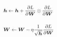
And SGD comparison , One more. h( Circles represent the multiplication of the corresponding matrix elements , Not dot product ).h Save the sum of squares of all previous gradient values . then , When updating parameters , By multiplying , You can adjust the scale of learning . It means , There are large changes in the elements of the parameter ( Greatly updated ) The learning rate of the elements will be smaller . in other words , The learning rate can be attenuated according to the elements of the parameter , Make the learning rate of parameters with large changes gradually decrease .
AdaGrad Will record the sum of squares of all gradients in the past . therefore , The deeper you study , to update The smaller the range . actually , If you study endlessly , The update amount will become 0, No more updates at all . To improve the problem , have access to RMSProp Method . RMSProp The method is not to add all the gradients in the past equally , But gradually Forget the gradient of the past , In addition, the information of the new gradient is more reflected . Professionally speaking, this kind of operation , be called “ Exponentially moving average ”, Decrease exponentially The scale of the past gradient .
Now let's implement it with code AdaDrad:
class AdaGrad:
    def __init__(self,lr = 0.01):
        self.lr = lr
        self.h = None

    def update(self,params,grads):
        if self.h is None:# initialization h
            self.h={
    }
            for key,val in params.items():
                self.h[key] = np.zeros_like(val)

        for key in params:
            self.h[key] += grads[key]*grads[key]
            params[key] -= self.lr*grads[key]/(np.sqrt(self.h[key])+1e-7)
            #1e-7 prevent 0 Used as the denominator
Same as Momentum Like drawing , Let's draw its path optimization diagram :
![[ Failed to transfer the external chain picture , The origin station may have anti-theft chain mechanism , It is suggested to save the pictures and upload them directly (img-RkqmhSsX-1644804304274)( 6、 ... and 、 Skills related to neural network learning .assets/ chart 6-12.png)]](/img/e2/82f3c89e24059ba12545d255465543.jpg)
Is the effect great ! The value of the function moves towards the minimum efficiently . because y Axial square The upward gradient is larger , Therefore, it has changed greatly at the beginning , But later, according to this larger change, press Adjust the proportion , Reduce the pace of updates . therefore ,y The update degree in the axis direction is weakened ,“ And ” The degree of change of the glyph is attenuated .
1.4 RMSprop
Because there is no explanation in the book , I suggest you look directly at Wu Enda's deeplearning About the exponential weighted average , A total of half an hour , No one should say better , So we have theories and don't know where to recommend watching his video . Remind everyone to pay attention to the explanation in the video β=0.9 It's the average temperature of ten days ,β=0.98 The time is 50 The average temperature of the day , You should understand why . Exponential weighted average is also called Exponentially moving average , And the essence of mobile is here . Give you a link , because b There are too many courses in Wu Enda , from p63 Start . Exponentially weighted average
After understanding the theory, directly use code to realize , and AdaGrad Only part of it is different .
class RMSprop:

    """RMSprop"""

    def __init__(self, lr=0.01, decay_rate = 0.99):
        self.lr = lr
        self.decay_rate = decay_rate
        self.h = None

    def update(self, params, grads):
        if self.h is None:
            self.h = {
    }
            for key, val in params.items():
                self.h[key] = np.zeros_like(val)

        for key in params.keys():
            self.h[key] *= self.decay_rate
            self.h[key] += (1 - self.decay_rate) * grads[key] * grads[key]
            params[key] -= self.lr * grads[key] / (np.sqrt(self.h[key]) + 1e-7)
![[ Failed to transfer the external chain picture , The origin station may have anti-theft chain mechanism , It is suggested to save the pictures and upload them directly (img-YG44Gon8-1644804304274)( 6、 ... and 、 Skills related to neural network learning .assets/ chart 6-15.png)]](/img/fb/c261367fa0b0b4c4e6f58356d740d9.jpg)
Here we use lr=0.1, The code in the book lr=0.01, however 0.01 The drawing is too far from the center point , Convergence is not enough , The rate of decline is α=0.98. Than the one above AdaGrad A little smooth .
1.5 Adam
Have studied computer network or operating system , When we design algorithms, we like stitching monsters best , Is to combine the two algorithms , At the same time, it has the advantages of both .
Momentum Move according to the physical rules of the ball rolling in the bowl ,AdaGrad For reference Adjust the update pace appropriately for each element of the number . What if these two methods are combined
Adam yes 2015 The new method proposed in . Its theory is a little complicated , Directly speaking , Is to melt All right Momentum and AdaGrad Methods . By combining the advantages of the previous two methods , Is expected to be Realize efficient search of parameter space . Besides , Carry out hyperparametric “ Offset correction ” It's also Adam Characteristics of . In Wu Enda's course RMSprop Then I'll talk about Adam 了 , It is suggested to go directly to this part of the theory class ,7 About minutes , Then come back to the code .
class Adam:


    def __init__(self, lr=0.001, beta1=0.9, beta2=0.999):
        self.lr = lr
        self.beta1 = beta1 # Momentum method parameters
        self.beta2 = beta2#RMSprop Parameters
        self.iter = 0
        self.m = None     # Momentum method
        self.v = None     #RMSprop Of

    def update(self, params, grads):
        if self.m is None:
            self.m, self.v = {
    }, {
    }
            for key, val in params.items():
                self.m[key] = np.zeros_like(val)
                self.v[key] = np.zeros_like(val)

        self.iter += 1
        lr_t = self.lr * np.sqrt(1.0 - self.beta2 ** self.iter) / (1.0 - self.beta1 ** self.iter)
        # Deviation correction lr_t  The learning rate and correction are calculated together

        for key in params.keys():
            self.m[key] = self.beta1*self.m[key] + (1-self.beta1)*grads[key]
            self.v[key] = self.beta2*self.v[key] + (1-self.beta2)*(grads[key]**2)
            #self.m[key] += (1 - self.beta1) * (grads[key] - self.m[key])# Teacher Wu Enda's method
            #self.v[key] += (1 - self.beta2) * (grads[key] ** 2 - self.v[key])# Teacher Wu Enda's method

            params[key] -= lr_t * self.m[key] / (np.sqrt(self.v[key]) + 1e-7)
You can observe that this is different from what Wu Enda said , In the calculation mt and vt One more hour is lost mt-1,vt-1, The following two lines of notes are the same as what Wu Enda said , The figures of these two calculation methods are drawn as follows
![[ Failed to transfer the external chain picture , The origin station may have anti-theft chain mechanism , It is suggested to save the pictures and upload them directly (img-Lk1VDKZ8-1644804304275)( 6、 ... and 、 Skills related to neural network learning .assets/ chart 6-13.png)]](/img/20/30fc681f47bdddaf9b41d392c932e3.jpg)
![[ Failed to transfer the external chain picture , The origin station may have anti-theft chain mechanism , It is suggested to save the pictures and upload them directly (img-pJKH8l8P-1644804304276)( 6、 ... and 、 Skills related to neural network learning .assets/ chart 6-16.png)]](/img/82/e786c53433f237dd9577889cf0c69c.jpg)
Have you found the same , So I guess the method in the book may be to correct another error that we haven't learned , But we can just follow what teacher Wu Enda said , After all, I don't see any difference between the two . The only thing that's hard to understand is in the code , The learning rate is multiplied by the two corrections , You can understand it with a push of a pen . Three or four line formula .
We introduced it above SGD、Momentum、AdaGrad、Adam,RMSprop this 5 Methods , that So which method is better ? Very regret ,( at present ) There is no such thing as being able to perform well in all problems Methods . this 4 Each method has its own characteristics , Both have their own problems that they are good at solving and are not good at solving The problem of . It is still used in many studies SGD.Momentum and AdaGrad It's also worth trying Methods . lately , Many researchers and technicians like to use Adam. In the future study, it is mainly used SGD and Adam.
边栏推荐
- Shopping malls, storerooms, flat display, user-defined maps can also be played like this!
- Selenium ide plug-in download, installation and use tutorial
- Review of enterprise security incidents: how can enterprises do a good job in preventing source code leakage?
- 高薪程序员&面试题精讲系列119之Redis如何实现分布式锁?
- Uniapp applet subcontracting
- tars源码分析之5
- Analysis of tars source code 1
- Download address of the official website of national economic industry classification gb/t 4754-2017
- Vulhub vulnerability recurrence 77_ zabbix
- [number theory] fast power (Euler power)
猜你喜欢
Vulhub vulnerability recurrence 76_ XXL-JOB
Industrial computer anti-virus

Uniapp applet subcontracting
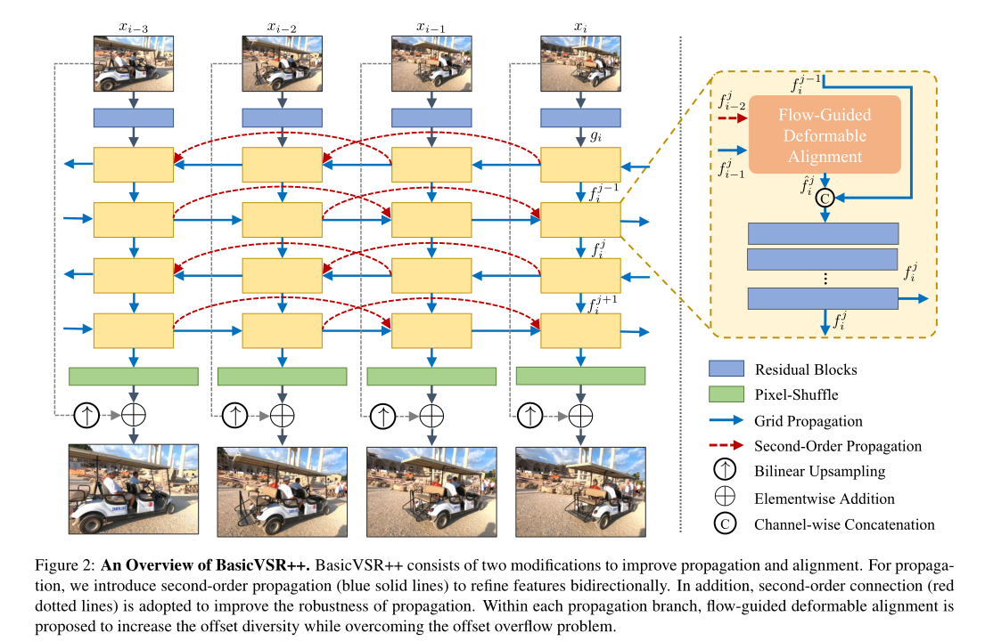
BasicVSR++: Improving Video Super-Resolutionwith Enhanced Propagation and Alignment

The most effective futures trend strategy: futures reverse merchandising
Cell reports: Wei Fuwen group of the Institute of zoology, Chinese Academy of Sciences analyzes the function of seasonal changes in the intestinal flora of giant pandas
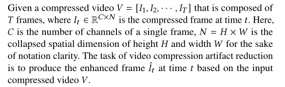
Recursive Fusion and Deformable Spatiotemporal Attention for Video Compression Artifact Reduction
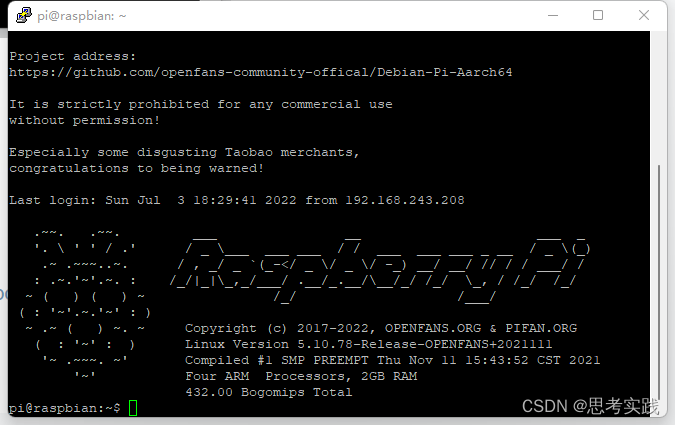
电脑通过Putty远程连接树莓派
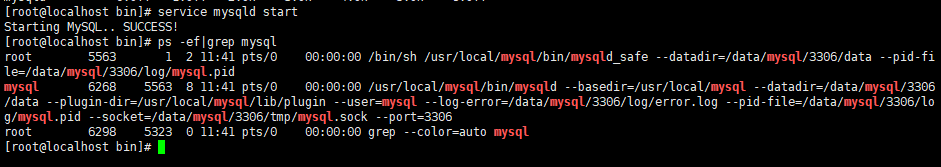
Centos8 install mysql 7 unable to start up

Deep profile data leakage prevention scheme
随机推荐
用于压缩视频感知增强的多目标网络自适应时空融合
校园网络问题
tars源码分析之10
js 常用时间处理函数
ABCD four sequential execution methods, extended application
Selenium driver ie common problem solving message: currently focused window has been closed
the input device is not a TTY. If you are using mintty, try prefixing the command with ‘winpty‘
What is tweeman's law?
【MySQL】数据库视图的介绍、作用、创建、查看、删除和修改(附练习题)
tars源码分析之4
Mysql 45讲学习笔记(七)行锁
Set JTAG fuc invalid to normal IO port
Data analysis notes 09
Tar source code analysis Part 3
Code rant: from hard coding to configurable, rule engine, low code DSL complexity clock
ABCD four sequential execution methods, extended application
uniapp小程序分包
[problem record] 03 connect to MySQL database prompt: 1040 too many connections
《剑指Offer》第2版——力扣刷题
Tar source code analysis Part 2