Numpy quick start (II) -- Introduction to array (creation of array + basic operation of array)

explain

• This article will not cover all array functions , And I won't explain all the parameters , For details, please refer to the official documents .
• With square brackets [ ] The parameters of can be omitted .
• The output of each small piece of code will be written in the comments below .

One 、 Array creation

1.1 Create an array with existing data

function	effect
np.array(object, dtype=None, copy=True)	object It can be Scalar 、 list 、 Tuples Objects such as ,dtype It's the data type ,copy Control whether to copy object; take object Convert to n Dimension group
np.asarray(object, dtype=None)	And np.array() Of Works in a similar way , See 1.1.2 section
np.fromfunction(f, shape, dtype=float)	shape It's a size of N Of Integer tuple ,f Yes. N Scalar function with parameters ; return shape Array of shapes , Each of these elements is passed in according to its index f The value after
np.fromstring(s, dtype=float, sep)	s Is string ,sep The separator is ; Convert a string into an array after splitting it by delimiters

1.1.1 np.array()

np.array() It's the most common way .

""" example 1 """
A = np.array([1, 2])
print(A)
print(type(A))
# [1 2]
# <class 'numpy.ndarray'>

""" example 2 """
A = np.array([(1, 2), (3, 4)])
print(A)
print(type(A))
# [[1 2]
# [3 4]]
# <class 'numpy.ndarray'>

""" example 3 """
A = np.array([1, 2, 3], dtype=np.complex128)
print(A)
# [1.+0.j 2.+0.j 3.+0.j]

""" example 4 """
A = np.array([1, 2, 3])
B = np.array(A)
print(B)
print(type(B))
# [1 2 3]
# <class 'numpy.ndarray'>

""" example 5 """
A = np.array([1, 2, 3])
B = np.array(A)
C = np.array(A, copy=False)
A[0] = 2
print(B, '\n', C)
# [1 2 3] 
# [2 2 3]

from example 4 It's not hard to find , our object It can also be ndarray.

from example 5 It can be seen that , If you turn off copy, We modify A The value of will affect C Of （ Because at this time C Point to A）. in fact , If A No ndarray（ Such as the list ）, So no matter copy Set to what , our np.array() Will make a copy of A.

1.1.2 np.asarray()

np.array() and np.asarray() Source data can be object Turn into ndarray, But the main difference is ： When the source data is ndarray when ,array Still will copy Make a copy , Occupy new memory , but asarray Can't .

The difference can be seen from the following two examples ：

""" example 1 """
A = [1, 2, 3]
B = np.array(A)
C = np.asarray(B)
A[0] = 2
print(A, '\n', B, '\n', C, sep='')
# [2, 2, 3] 
# [1 2 3] 
# [1 2 3]

""" example 2 """
A = np.array([1, 2, 3])
B = np.array(A)
C = np.asarray(A)
A[0] = 2
print(A, '\n', B, '\n', C, sep='')
# [2 2 3] 
# [1 2 3] 
# [2 2 3]

For the convenience of memory , We can think of it this way ：

#  Loosely speaking , The following two statements are equivalent ：
np.array(object, copy=False)
np.asarray(object)

If there is no special need , Use as much as possible np.array() instead of np.asarray().

1.1.3 np.fromfunction()

Let's first define a function

def f(x, y):
    return x + y

because f There are two parameters , therefore shape The size of should also be 2. Let's set up shape=(3, 2), Then the final returned size is $3\times 2$ Array of . Remember that the array is $A$, So naturally

$$A[i][j]=f(i,j)=i+j$$

Let's take a look at the effect ：

A = np.fromfunction(f, (3, 2), dtype=int)
print(A)
# [[0 1]
# [1 2]
# [2 3]]

If you use python Is an anonymous function of , We only need one line of code ：

A = np.fromfunction(lambda x, y: x + y, (3, 2), dtype=int)

Use np.fromfunction(), We can easily create an array of elements related to the index , for example , For the following array ：

$$\left[\begin{array}{ccc}\mathrm{T}\mathrm{r}\mathrm{u}\mathrm{e}& \mathrm{F}\mathrm{a}\mathrm{l}\mathrm{s}\mathrm{e}& \mathrm{F}\mathrm{a}\mathrm{l}\mathrm{s}\mathrm{e}\\ \mathrm{F}\mathrm{a}\mathrm{l}\mathrm{s}\mathrm{e}& \mathrm{T}\mathrm{r}\mathrm{u}\mathrm{e}& \mathrm{F}\mathrm{a}\mathrm{l}\mathrm{s}\mathrm{e}\\ \mathrm{F}\mathrm{a}\mathrm{l}\mathrm{s}\mathrm{e}& \mathrm{F}\mathrm{a}\mathrm{l}\mathrm{s}\mathrm{e}& \mathrm{T}\mathrm{r}\mathrm{u}\mathrm{e}\end{array}\right]$$

We can create ：

A = np.fromfunction(lambda i, j: i == j, (3, 3))

1.1.4 np.fromstring()

For the following string ：

s = '1 2 3 4 5'

To convert it to an integer array , Our first reaction was ：

A = np.array(list(map(int, s.split())))
print(A)
# [1 2 3 4 5]

But use np.fromstring(), We can create it more easily . Notice that each number in the string is separated by a space , So just set up sep=’ ' that will do ：

A = np.fromstring(s, dtype=int, sep=' ')
print(A)
# [1 2 3 4 5]

1.2 Create an array based on the range of values

function	effect
np.arange([start], stop, [step], dtype=None)	Create one in [ start, stop ) In the interval , In steps of step Array of ;start When omitted, the default is 0,step When omitted, the default is 1
np.linspace(start, stop, num=50, endpoint=True, dtype=None)	Create one in [ start, stop ] In the interval , The size is num Array of ; When endpoint closed , The interval becomes [ start, stop )
np.logspace(start, stop, num=50, endpoint=True, base=10.0, dtype=None)	Equivalent to the np.linspace() Based on the results , For each of these elements $a$ Make a change $a:=bas{e}^a$
np.geomspace(start, stop, num=50, endpoint=True, dtype=None)	And np.logspace() similar , It's just np.geomspace() The appropriate substrate will be automatically selected

1.2.1 np.arange()

""" example 1 """
A = np.arange(6)
B = np.arange(2, 6)
C = np.arange(2, 10, 2)
print(A, '\n', B, '\n', C, sep='')
# [0 1 2 3 4 5]
# [2 3 4 5]
# [2 4 6 8]

""" example 2 """
A = np.arange(6, -1, -1, dtype=float)
print(A)
# [6. 5. 4. 3. 2. 1. 0.]

""" example 3 """
A = np.arange(6, -1, -1.0)
print(A)
# [6. 5. 4. 3. 2. 1. 0.]

Be careful ： When start The value of is much greater than step The value of ,np.arange() It may not return the expected results , You need to use np.linspace() 了

1.2.2 np.linspace()

np.linspace() By default, the floating-point array is returned （float_）

""" example 1 """
A = np.linspace(1, 10, 10)
B = np.linspace(1, 10, 10, endpoint=False)
print(A, '\n', B, sep='')
# [ 1. 2. 3. 4. 5. 6. 7. 8. 9. 10.]
# [1. 1.9 2.8 3.7 4.6 5.5 6.4 7.3 8.2 9.1]

1.2.3 np.logspace()

The function and np.linspace() Functions are closely related , Let's see first np.linspace() An example of ：

A = np.linspace(1, 5, 5)
print(A)
# [1. 2. 3. 4. 5.]

take linspace Replace with logspace, And set the base to 2：

A = np.logspace(1, 5, 5, base=2)

According to the description in the previous table , The result should be ：

$$[2^1,2^2,2^3,2^4,2^5]$$

The output is also true ：

# [ 2. 4. 8. 16. 32.]

1.2.4 np.geomspace()

np.logspace() and np.geomspace() Will generate an exponentially growing array , The difference lies in ,logspace The resulting array is ：

$$[bas{e}^{start},\cdots ,bas{e}^{stop}]$$

and geomspace The resulting array is ：

$$[start,\cdots ,stop]$$

for example , Set up start=1,stop=1000,num=4, be geomspace The base will be automatically selected 10：

A = np.geomspace(1, 1000, num=4, dtype=int)
print(A)
# [ 1 10 100 1000]

1.3 Create an array of a specific type

function	effect
np.empty(shape)	shape by Integers or Integer list / Tuples ; return shape The shape of the An empty array （ Uninitialized array ）
np.empty_like(prototype)	prototype Is a given array ; Returns an array corresponding to the given array The same shape Of An empty array
np.ones(shape)	return shape The shape of the whole 1 Array
np.ones_like(prototype)	Returns an array with a given The same shape Of whole 1 Array
np.zeros(shape)	return shape The shape of the whole 0 Array
np.zeros_like(prototype)	Returns an array with a given The same shape Of whole 0 Array
np.full(shape, value)	value by Scalar or Array ; When value When it's scalar , Return one with shape Of the same shape whole value Array ;value See 1.3.4 section
np.full_like(prototype, value)	Returns an array with a given The same shape Of whole value Array
np.eye(m, n=m, k=0)	m It's the number of rows in the matrix ,n It's the number of columns in a matrix ,k Control diagonal ; return The main diagonal is all 1, The rest are 0 Matrix （ Array ）
np.identity(n)	return n rank Unit matrix

1.3.1 np.empty()

empty And zeros Different , it Can't Initialize element to 0（ But it doesn't mean that there are no numbers in the array ）, So the speed may be faster than zeros faster .

""" example 1 """
A = np.empty(2)
print(A)
# [4.64929150e+143 2.37662553e-045]

""" example 2 """
A = np.empty([2, 2])
print(A)
# [[ 1.05328699e-311 -6.77097176e-233]
# [ 1.05328694e-311 1.05328694e-311]]

""" example 3 """
A = np.array([1, 2, 3])
B = np.empty_like(A)
print(B)
# [5111887 5701703 5111877]

1.3.2 np.ones()

""" example 1 """
A = np.ones([2, 2])
print(A)
# [[1. 1.]
# [1. 1.]]

""" example 2 """
A = np.array([1, 2, 3])
B = np.ones_like(A)
print(B)
# [1 1 1]

1.3.3 np.zeros()

""" example 1 """
A = np.zeros(5)
print(A)
# [0. 0. 0. 0. 0.]

""" example 2 """
A = np.array([1, 2, 3])
B = np.zeros_like(A)
print(B)
# [0 0 0]

1.3.4 np.full()

""" example 1 """
A = np.full((2, 3), 3)
print(A)
# [[3 3 3]
# [3 3 3]]

""" example 2 """
A = np.full((3, 3), [1, 2, 3])
print(A)
# [[1 2 3]
# [1 2 3]
# [1 2 3]]

It can be seen that , When value When it's an array , Each row in the returned array is used value Filled . It should be noted that , In this case ,shape[1] Need and len(value) bring into correspondence with , Otherwise, an error will be reported ：

A = np.full((3, 4), [1, 2, 3])
print(A)
# ValueError: could not broadcast input array from shape (3,) into shape (3,4)

Let's see np.full_like()：

A = np.arange(6, dtype=int)
B = np.full_like(A, 1)
C = np.full_like(A, 0.1)
D = np.full_like(A, 0.1, dtype=float)
print(A, '\n', B, '\n', C, '\n', D, sep='')
# [0 1 2 3 4 5]
# [1 1 1 1 1 1]
# [0 0 0 0 0 0]
# [0.1 0.1 0.1 0.1 0.1 0.1]

1.3.5 np.eye()

First introduce the diagonal .

The main diagonal ：

$$(0,0)\to (1,1)\to \cdots \to (s,s)$$

for example , In the following two matrices ,1 The paths are the main diagonal ：

$$\left[\begin{array}{cc}1& 0\\ 0& 1\end{array}\right],\left[\begin{array}{ccc}1& 0& 0\\ 0& 1& 0\end{array}\right]$$

Sub diagonal ：

$$\begin{gathered} \mathrm{T}\mathrm{y}\mathrm{p}\mathrm{e}\mathrm{I}:(0,0+k)\to (1,1+k)\to \cdots \to (s,s+k),k\ge 1 \\ \mathrm{T}\mathrm{y}\mathrm{p}\mathrm{e}\mathrm{I}\mathrm{I}:(0-k,0)\to (1-k,1)\to \cdots \to (s-k,s),k\le -1 \end{gathered}$$

among $k$ Is an integer .

Let's first look at the first diagonal , You might as well set $k=1$, The path is

$$(0,1)\to (1,2)\to (2,3)\to \cdots \to (s,s+1)$$

for example , In the following two matrices ,1 The paths are the first type of sub diagonal ：

$$\left[\begin{array}{ccc}0& 1& 0\\ 0& 0& 1\\ 0& 0& 0\end{array}\right],\left[\begin{array}{ccccc}0& 1& 0& 0& 0\\ 0& 0& 1& 0& 0\\ 0& 0& 0& 1& 0\end{array}\right]$$

It is equivalent to the upward translation of the main diagonal $k$ Units get the first type of sub diagonal .

Look at the second diagonal , Might as well set $k=-1$, The path is ：

$$(1,0)\to (2,1)\to (3,2)\to \cdots \to (s+1,s)$$

for example , In the following two matrices ,1 The paths are all type II sub diagonal ：

$$\left[\begin{array}{ccc}0& 0& 0\\ 1& 0& 0\\ 0& 1& 0\end{array}\right],\left[\begin{array}{ccc}0& 0& 0\\ 1& 0& 0\\ 0& 1& 0\\ 0& 0& 1\\ 0& 0& 0\end{array}\right]$$

It is equivalent to the downward translation of the main diagonal $-k$ Units get the second type of sub diagonal .

So we can make a summary ：

• $k=0$ Time is the main diagonal .
• $k>0$ It is the first type of sub diagonal , It is equivalent to the upward translation of the main diagonal $k$ Three units get .
• $k<0$ It is the second type of sub diagonal , It is equivalent to the downward translation of the main diagonal $-k$ Three units get .

For convenience , We all use it “ The first $k$ Diagonals ” This name is used to call all diagonals . for example , The first $0$ This diagonal is the main diagonal , The first $1$ Diagonal lines are translated upward from the main diagonal 1 Three units get , The first $-1$ Diagonal lines are translated downward from the main diagonal 1 Three units get .

After knowing what diagonal is , The following example is not difficult to understand ：

""" example 1 """
A = np.eye(3)
print(A)
# [[1. 0. 0.]
# [0. 1. 0.]
# [0. 0. 1.]]

""" example 2 """
A = np.eye(3, 5)
print(A)
# [[1. 0. 0. 0. 0.]
# [0. 1. 0. 0. 0.]
# [0. 0. 1. 0. 0.]]

""" example 3 """
A = np.eye(3, 4, k=2)
print(A)
# [[0. 0. 1. 0.]
# [0. 0. 0. 1.]
# [0. 0. 0. 0.]]

""" example 4 """
A = np.eye(5, 3, k=-3)
print(A)
# [[0. 0. 0.]
# [0. 0. 0.]
# [0. 0. 0.]
# [1. 0. 0.]
# [0. 1. 0.]]

1.3.6 np.identity()

The following three statements are equivalent ：

np.eye(n)
np.eye(n, n)
np.identity(n)

1.4 Create diagonal matrix 、 On / Lower triangular matrix

function	effect
np.diag(v, k=0)	k Control diagonal ; When v When it is a two-dimensional array , The first k Diagonal lines are returned as a one-dimensional array ; When v Is a one-dimensional array , This array will be used as the k Diagonal lines and construct diagonal matrix
np.tri(m, n=m, k=0)	Create a m×n Matrix , Among them the first k Diagonals And the following Part of All for 1, Other locations All for 0
np.tril(object, k=0)	object Is a two-dimensional array ; Return to one object Copy of , Among them, the copy is k Diagonals above Part of Set as 0
np.triu(object, k=0)	Return to one object Copy of , Among them, the copy is k Diagonals following Part of Set as 0

1.4.1 np.diag()

""" example 1 """
A = np.array([[1, 2], [3, 4]])
print(np.diag(A))
print(np.diag(A, k=1))
# [1 4]
# [2]

""" example 2 """
A = np.array([1, 2, 3])
print(np.diag(A))
print(np.diag(A, k=1))
# [[1 0 0]
# [0 2 0]
# [0 0 3]]
# [[0 1 0 0]
# [0 0 2 0]
# [0 0 0 3]
# [0 0 0 0]]

1.4.2 np.tri()

""" example 1 """
A = np.tri(3, 4, k=1)
print(A)
# [[1. 1. 0. 0.]
# [1. 1. 1. 0.]
# [1. 1. 1. 1.]]

""" example 2 """
A = np.tri(3, 4, k=-1)
print(A)
# [[0. 0. 0. 0.]
# [1. 0. 0. 0.]
# [1. 1. 0. 0.]]

""" example 3 """
A = np.tri(2, k=-1)
print(A)
# [[0. 0.]
# [1. 0.]]

1.4.3 np.tril()

""" example 1 """
A = np.array([[1, 2, 3], [4, 5, 6], [7, 8, 9]])
print(np.tril(A))
# [[1 0 0]
# [4 5 0]
# [7 8 9]]

""" example 2 """
A = np.array([[1, 2, 3], [4, 5, 6], [7, 8, 9]])
print(np.tril(A, k=-1))
# [[0 0 0]
# [4 0 0]
# [7 8 0]]

1.4.4 np.triu()

""" example 1 """
A = np.array([[1, 2, 3], [4, 5, 6], [7, 8, 9]])
print(np.triu(A))
# [[1 2 3]
# [0 5 6]
# [0 0 9]]

""" example 2 """
A = np.array([[1, 2, 3], [4, 5, 6], [7, 8, 9]])
print(np.triu(A, k=1))
# [[0 2 3]
# [0 0 6]
# [0 0 0]]

Two 、 Basic operations of arrays

2.1 Look at the array information

We already know , stay Numpy in , One dimensional array represents vector , Two dimensional array representation matrix , For three-dimensional and above arrays , We're going to use it tensor Here we are .

stay Numpy in , The dimension of the array has another name —— Axis （axes）, A few dimensional array has several axes . for example , For the following two-dimensional array ：

[[0., 0., 0.],
 [1., 1., 1.]]

It has two axes , And the length of the array along the first axis is 2, The length along the second axis is 3, namely ：

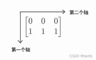
See here you may wonder , Why? The first axis is along the row direction and the second axis is along the column direction ？ Why not make the first axis follow the column direction and the second axis follow the row direction ？

This is because , When we index , The index is in the form of $A[i][j]$. That's ok The index is on page One A place , Column The index is on page Two A place , So our first axis is defined as along the line , The second axis is specified along the column direction .

about N Dimension group , We also call it N For the array Rank （rank）.

We have the following methods to view the information of the array ：

Method	effect
ndarray.ndim	Returns the... Of the array dimension （ Rank ）
ndarray.shape	With Tuples Form returns the shape of the array ; For example, for a two-dimensional array , The returned form is (m, n)
ndarray.size	Returns the value of an element in an array total ; This is equal to shape The product of all elements in
ndarray.dtype	Returns the... Of the array data type （ Because the array requires that the data type of all elements in it must be the same ）

We will learn more about these methods through an example ：

A = np.array([[1, 2, 3], [4, 5, 6]])
print(A.ndim)
print(A.shape)
print(A.size)
print(A.dtype)
# 2
# (2, 3)
# 6
# int32

2.2 Arithmetic operator

Applying arithmetic operators to arrays will By element （ Also called element by element ） To deal with .

A = np.array([1, 2, 3])
B = np.array([4, 5, 6])

print(A + B)
# [5 7 9]
print(B - A)
# [3 3 3]
print(A + 2)
# [3 4 5]
print(A * 2)
# [2 4 6]
print(A / 2)
# [0.5 1. 1.5]
print(A ** 2)
# [1 4 9]
print(A * B)
# [ 4 10 18]
print(A ** B)
# [ 1 32 729]
print(A >= 2)
# [False True True]

When it comes to different accuracy （ data type ） Array of , The accuracy of the results （ data type ） For the array involved in the operation Highest accuracy （ Upward conversion ）.

for example , The data types are int32 and float64 Add the two arrays of , The result will be an accuracy of float64 Array of ：

A = np.array([1, 2, 3], dtype=int)
B = np.array([4, 5, 6], dtype=float)
C = A + B
print(C)
print(C.dtype)
# [5. 7. 9.]
# float64

The data types are float64 and complex128 Add the two arrays of , The result will be an accuracy of complex128 Array of ：

A = np.array([1, 2, 3], dtype=complex)
B = np.array([4, 5, 6], dtype=float)
C = A + B
print(C)
print(C.dtype)
# [5.+0.j 7.+0.j 9.+0.j]
# complex128

2.3 Index and slice

Numpy Of n Dimension groups can be like Python Index like a list of 、 assignment 、 section 、 Iteration and so on .

2.3.1 Indexes （indexing）

n The method of indexing and assigning dimension groups is the same as that of lists ：

A = np.arange(12)
print(A[3])
# 3
A[5] = 9
print(A)
# [ 0 1 2 3 4 9 6 7 8 9 10 11]

Of course, we can index multiple elements at the same time ：

A = np.arange(12)
indexes_1 = np.array([1, 4, 7, 9])
indexes_2 = [1, 4, 7, 9]
print(A[indexes_1])
print(A[indexes_2])
# [1 4 7 9]
# [1 4 7 9]

It can be seen that ,indexes by n Dimension group or list Can complete the indexing of multiple elements , but indexes Indexing fails when it is a tuple .

For a two-dimensional list , The method of indexing an element is $A[i][j]$. But in a two-dimensional array , In addition to this method , There is another way ：$A[i,j]$.

A = np.array([[1, 2, 3], [4, 5, 6]])
print(A[0, 1])
print(A[1, -1])
# 2
# 6

Please use $A[i,j]$, It's more efficient than $A[i][j]$ Higher .

If the index number is less than the dimension of the array , You will get a sub array ：

A = np.array([[1, 2, 3], [4, 5, 6]])
print(A[0]) #  It's equivalent to taking A Of the 0 That's ok 
# [1 2 3]

Back to the one-dimensional array , If the array capacity is very large , And when we need to index many elements , Is there a simpler method ？

The answer is slicing .

2.3.2 section （slicing）

• More than n Dimension groups and lists ,python Any ordered sequence in supports slicing , Such as a string , Tuples etc. .
• The result type returned by slicing is consistent with the type of the sliced object . Slice the array to get the array , Slice the list to get the list , Slice the string to get the string .

We will only discuss array slicing next , Its standard format is ：

$$A[start:stop:step],step\ne 0$$

start Is the slice start index ,end Is the slice end index , Notice that this is Left closed right away Section , namely $[start,stop)$.

step When omitted The default is 1, And step The symbol of determines the slice Direction ：step Positive timing , Perform forward slicing ;step When it is negative , Perform reverse slicing .

for example ：

A = np.arange(10)
print(A[1:6:1])
print(A[5:0:-1])
# [1 2 3 4 5]
# [5 4 3 2 1]

hypothesis step Given ：

• If only omitted stop, Will follow start Start slicing in the direction of slicing to an end of the array （ Include endpoints ）.
• If only omitted start, It will slice from one end of the array along the slice direction to stop（ It doesn't contain stop）.

for example ：

A = np.arange(10)
print(A[1::1])
print(A[:0:-1])
# [1 2 3 4 5 6 7 8 9]
# [9 8 7 6 5 4 3 2 1]

• if start and stop All omitted , Then it will slice from one end of the array along the slice direction to the other end （ Include endpoints ）

for example ：

A = np.arange(10)
print(A[::1])
print(A[::-1])
# [0 1 2 3 4 5 6 7 8 9]
# [9 8 7 6 5 4 3 2 1 0]

So we got a fast Inversion array Methods ：

A = A[::-1]

because step by 1 You can omit , And you can further omit a colon , That is, the following three statements are equivalent ：

A[start:stop:1]
A[start:stop:]
A[start:stop]

So we can still get one Copy the array Methods ：

B = A[:]

After getting familiar with slicing , We can complete more complex operations , For example, for the following matrix ：

$$A=\left[\begin{array}{cccc}1& 2& 3& 4\\ 5& 6& 7& 8\\ 9& 10& 11& 12\\ 13& 14& 15& 16\end{array}\right]$$

If we want to take out $A$ The last three lines of , You can do this ：

#  The following two statements are equivalent , Try to think about why equivalence 
print(A[1:, :])
print(A[1:])

If we want to take out $A$ The last three columns of , This should be done ：

#  Try to think about why there is only one solution 
print(A[:, 1:])

To get $2,4,10,12$ These four elements , We only need to index as follows （ section ）：

#  It's equivalent to taking the first place 0 That's ok 、 The first 3 Lines and 1 Column 、 The first 3 Elements where columns intersect 
print(A[::2, 1::2])
# [[ 2 4]
# [10 12]]

2.3.3 Advanced index

In this section, we will discuss more advanced indexing （ section ）, It can help you select some elements easily and quickly .

2.3.3.1 Ellipsis （…） Use

go back to 2.3.1 section , We know , For a two-dimensional array , Take it out along The first axis In the direction of first Subarray （ Take the first 0 That's ok ）, You should use A[0], in fact , It is equivalent to A[0, :]. For three-dimensional arrays , Take its third... In the direction of the third axis k Subarray , We should use A[:, :, k], At this time, we have no more concise expression .

So here comes the question , about N Dimension group , When N Very big time , If we want to take its number on an axis k Subarray , Our index will cover Lots of colons and commas , And manual input is unrealistic , How to solve this problem ？

Fortunately Numpy Provides a more concise representation , When there is Two or more Colon of , We can use three points ... Instead of . for example , For the second example above , We can write simply A[..., k].

If A Is a five dimensional array , be ：

• A[1,2,...] Equivalent to A[1,2,:,:,:]
• A[...,3] Equivalent to A[:,:,:,:,3]
• A[4,...,5,:] Equivalent to A[4,:,:,5,:]

Ellipsis ... In the index Once at most .

Let's look at an example of a three-dimensional array ：

A = np.array([[[0, 1, 2], 
			   [10, 12, 13]], 
			  [[100, 101, 102],
			   [110, 112, 113]]])
print(A[1, :, :])
print(A[1, ...])
# [[100 101 102]
# [110 112 113]]
# [[100 101 102]
# [110 112 113]]

print(A[..., 2])
# [[ 2 13]
# [102 113]]

2.3.3.2 Use index array to index

stay 2.3.1 In section, we mentioned , have access to n Dimension group or list Finish indexing multiple elements . To be closer Numpy, Next, let's discard the list , Use only n Dimension group de indexing . This method is also called using index array to index .

Let's start with a simple example ：

A = np.arange(12)
i = np.array([0, 1, 4, 7])
print(A[i])
# [0 1 4 7]

When our index array is a two-dimensional array , The returned result is also a two-dimensional array ：

A = np.arange(12)
i = np.array([[0, 1], [4, 7]])
print(A[i])
# [[0 1]
# [4 7]]

We can extend it mathematically to a more general form , hypothesis indexes yes $k$ Dimension group , namely ：

$$indexes[i_1,i_2,\cdots ,i_k]=a_{i_1{i}_2\cdots i_k}$$

Thus, the results after indexing A[indexes] Satisfy ：

$$A[indexes][i_1,i_2,\cdots ,i_k]=A[a_{i_1{i}_2\cdots i_k}]$$

We can also provide multiple indexes for , But pay attention to the index array of each dimension Must have the same shape ：

A = np.array([[0, 1, 2, 3], 
			  [4, 5, 6, 7], 
			  [8, 9, 10, 11]])

i = np.array([[0, 1], 
			  [1, 2]])
j = np.array([[2, 1], 
			  [3, 3]])

print(A[i, j])
# [[ 2 5]
# [ 7 11]]

print(A[i, 2])
# [[ 2 6]
# [ 6 10]]

print(A[i, :])
# [[[ 0 1 2 3]
# [ 4 5 6 7]]
# [[ 4 5 6 7]
# [ 8 9 10 11]]]

Since we can index multiple elements , Then we should also be able to complete Assignment of multiple elements ：

""" example 1 """
A = np.array([0, 1, 2, 3, 4])
A[[0, 1, 3]] = 5
print(A)
# [5 5 2 5 4]

""" example 2 """
A = np.array([0, 1, 2, 3, 4])
A[[0, 1, 3]] = [7, 8, 9]
print(A)
# [7 8 2 9 4]

""" example 3 """
A = np.array([0, 1, 2, 3, 4])
A[[0, 1, 3]] = A[[0, 1, 3]] + 1
print(A)
# [1 2 2 4 4]

""" example 4 """
A = np.array([0, 1, 2, 3, 4])
A[[0, 0, 3]] += 1
print(A)
# [1 1 2 4 4]

You can see ,example 4 in ,$0$ Value Only once , Why? ？

This is because ,A[[0, 0, 3]] Itself is [0, 0, 3], perform A[[0, 0, 3]] += 1 Equivalent to execution A[[0, 0, 3]] = A[[0, 0, 3]] + 1 , It is equivalent to executing A[[0, 0, 3]] = [1,1,4], This statement is equivalent to

A[0] = 1
A[0] = 1
A[3] = 4

It can be seen that A[0] Assigned repeatedly , Therefore, its value will not increase twice .

So if we want A[0] The value of is increased twice （ In maintaining A[3] Only increase once ）, How do you do that ？

We only need to modify the assignment :

A[[0, 0, 3]] += [x, 2, 1]

among x It can be any number , Because then A[0] The value of will be 2 Cover . The above statement is equivalent to ：

A[0] = x
A[0] = 2
A[3] = 1

2.3.3.3 Index using Boolean arrays

Let's start with an example ：

A = np.array([[1, 2, 3], 
			  [4, 5, 6]])
i = np.array([[True, False, False], 
			  [False, False, True]])
print(A[i])
# [1 6]

It can be seen that , We only indexed True The place of , But for False Where there is no index .

Take advantage of this feature , We can do some interesting operations . for example , For the above array A, If you want to let A Medium greater than or equal to 3 All elements are set to 0, We can create a Boolean array first , Subsequent assignment ：

A = np.array([[1, 2, 3], [4, 5, 6]])
i = A >= 3
print(i)
# [[False False True]
# [ True True True]]

A[i] = 0
print(A)
# [[1 2 0]
# [0 0 0]]

Let's look at a few more examples to further familiarize ourselves with Boolean array indexes ：

A = np.array([[1, 2, 3], 
		      [5, 6, 7]])
i = np.array([False, True])
j = np.array([True, False, True])

print(A[i, :])
# [[5 6 7]]

print(A[:, j])
# [[1 3]
# [5 7]]

print(A[i, j])
# [5 7]

2.4 Broadcast mechanism （broadcasting）

Numpy When dealing with two or more arrays of different shapes Broadcast mechanism . simply , Namely Expand One of the arrays or At the same time expand Two arrays make their The same shape , In this way, the operation can continue .

2.4.1 Scalar and one-dimensional array

for example , Scalar * Array In this operation , We adopted the broadcasting mechanism ：

a = np.array([1, 2, 3])
b = 2
print(a * b)
# [2 4 6]

In the calculation A * b when ,Numpy Will b Expand to and A An array of the same size then performs the operation by element （ Arithmetic operators operate on elements , The operation by element requires the same shape of the two arrays ）：

When Big （ shape ） Array and Small （ shape ） Array operation , Small array will pass Copy yourself Expand into and large arrays The same shape Array of , This process is called radio broadcast . Later we will know , Not all arrays can be broadcast .

For the example above , We can do the same thing ：

a = np.array([1, 2, 3])
b = np.array([2, 2, 2])
print(a * b)

Their results are the same , But using broadcast mechanism is undoubtedly better , Because the broadcast mechanism takes up less memory space , And it is more convenient to use .

2.4.2 One dimensional arrays and two-dimensional arrays

consider One dimensional array + Two dimensional array The circumstances of , because + It's an arithmetic operator , You need to By element operation , But their shapes are different , therefore Numpy Will adopt the broadcasting mechanism ： A one-dimensional array expands into an array with the same shape as a two-dimensional array by copying itself .

a = np.array([[0, 0, 0], 
			  [10, 10, 10], 
			  [20, 20, 20], 
			  [30, 30, 30]])
b = np.array([1, 2, 3])
print(a + b)
# [[ 1 2 3]
# [11 12 13]
# [21 22 23]
# [31 32 33]]

The specific broadcasting process is as follows ：

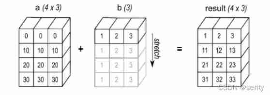
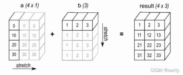
there b It's a line vector , So it will Along the line Broadcast （ namely Down ）; If b Is a column vector , Meeting Along the column Broadcast （ namely towards the right ）.

a = np.array([[0, 0, 0], 
			  [10, 10, 10], 
			  [20, 20, 20], 
			  [30, 30, 30]])
b = np.array([[1], 
			  [2], 
			  [3], 
			  [4]])
print(a + b)
# [[ 1 1 1]
# [12 12 12]
# [23 23 23]
# [34 34 34]]

The specific schematic diagram is not given here , Please imagine for yourself .

2.4.3 One dimensional array （ Column vector ） And one-dimensional array （ Row vector ）

consider Column vector + Row vector The circumstances of , here Numpy Meeting At the same time Two arrays , Put it all After expanding into a two-dimensional array , Then add by element .

a = np.array([[0],
			  [10],
			  [20],
			  [30]])
b = np.array([1, 2, 3])
print(a + b)
# [[ 1 2 3]
# [11 12 13]
# [21 22 23]
# [31 32 33]]

The specific broadcasting process is as follows ：

2.4.4 Broadcasting rules

See here , Readers may wonder , When can it be broadcast and when can it not be broadcast ？

take it easy , So let's look down .

For one N For dimensional arrays , It has N Axes . We use shape Method can get its shape , And in the form of tuples ：$(a_1,a_2,\cdots ,a_N)$, For the convenience of narration , We express it as

$$a_1\times a_2\times \cdots \times a_N\text{\hspace{1em}(A)}$$

For example, for a $5$ That's ok $3$ Columns of the matrix （ Two dimensional array ）, Its shape is $5\times 3$.

Now consider M An array of dimensions （ among $M<N$）, Its shape is

$$b_1\times b_2\times \cdots \times b_M$$

by Ensure that the subscripts are consistent after right alignment , We change the subscript of the above formula ：

$$b_k\times b_{k+1}\times \cdots \times b_N\text{\hspace{1em}(B)}$$

There should be $N-k+1=M$, namely $k=N-M+1\ge 2$.

Now we will $(B)$ Arranged in $(A)$ Type below And implement Right alignment , Then there are ：

$$\begin{array}{rl}{a}_1\times a_2\times \cdots \times & a_k\times a_{k+1}\times \cdots \times a_N\\ & b_k\times b_{k+1}\times \cdots \times b_N\end{array}$$

Here we give a definition ：$(a_i,b_i)$ be called Compatible Of , If and only if $a_i=b_i$ or $a_i$ and $b_i$ One of them is $1$.

So we got it Broadcasting rules ： if $(a_i,b_i),k\le i\le N$ It's all Compatible Of , be M Dimension groups can be broadcast .

As defined above , The result after broadcasting is

$$a_1\times \cdots \times a_{k-1}\times \max (a_k,b_k)\times \max (a_{k+1},b_{k+1})\times \cdots \times \max (a_N,b_N)$$

Let's consolidate this concept with a few examples ：

"""  It's broadcast  """
A      (4d array):  8 x 1 x 6 x 1
B      (3d array):      7 x 1 x 5
Result (4d array):  8 x 7 x 6 x 5

A      (2d array):  5 x 4
B      (1d array):      1
Result (2d array):  5 x 4

A      (2d array):  5 x 4
B      (1d array):      4
Result (2d array):  5 x 4

A      (3d array):  15 x 3 x 5
B      (3d array):  15 x 1 x 5
Result (3d array):  15 x 3 x 5

A      (3d array):  15 x 3 x 5
B      (2d array):       3 x 5
Result (3d array):  15 x 3 x 5

A      (3d array):  15 x 3 x 5
B      (2d array):       3 x 1
Result (3d array):  15 x 3 x 5

"""  Not broadcast  """
A      (1d array):  3
B      (1d array):  4 

A      (2d array):      2 x 1
B      (3d array):  8 x 4 x 3 

When there is a situation that cannot be broadcast , The program will report an error ：ValueError: operands could not be broadcast together with shapes ...