当前位置:网站首页>[the Nine Yang Manual] 2017 Fudan University Applied Statistics real problem + analysis
[the Nine Yang Manual] 2017 Fudan University Applied Statistics real problem + analysis
2022-07-06 13:30:00 【Elder martial brother statistics】
Catalog
The real part
One 、(30 branch ) A term is used to explain
(1)(5 branch ) Sample mean 、 Sample variance ;
(2)(5 branch ) statistic ;
(3)(5 branch ) Order statistics ;
(4)(5 branch ) Median 、 Sample median ;
(5)(5 branch ) Empirical distribution function ;
(6)(5 branch ) Unbiased estimate .
Two 、(20 branch ) X 1 , X 2 , X_{1}, X_{2}, X1,X2, i.i.d ∼ Exp ( 1 ) , \sim \operatorname{Exp}(1), ∼Exp(1), seek
(1)(10 branch ) X 1 X 1 + X 2 \frac{X_{1}}{X_{1}+X_{2}} X1+X2X1 Density function of ;
(2)(10 branch ) X ( 2 ) − X ( 1 ) X_{(2)}-X_{(1)} X(2)−X(1) Density function of .
3、 ... and 、(20 branch ) X 1 , X 2 X_{1}, X_{2} X1,X2 i.i.d. ∼ N ( 0 , 1 ) , \sim N(0,1), ∼N(0,1), seek X 1 X 2 \frac{X_{1}}{X_{2}} X2X1 Probability distribution of .
Four 、(20 branch ) X 1 , X 2 , … , X n X_{1}, X_{2}, \ldots, X_{n} X1,X2,…,Xn i.i.d. ∼ F ( x ) , \sim F(x), ∼F(x), remember Y n ( x ) = ∑ i = 1 n I [ X i ≤ x ] , Y_{n}(x)=\sum_{i=1}^{n} I\left[X_{i} \leq x\right], Yn(x)=∑i=1nI[Xi≤x], seek lim n → ∞ Y n ( x ) n \lim _{n \rightarrow \infty} \frac{Y_{n}(x)}{n} limn→∞nYn(x).
5、 ... and 、(20 branch ) X 0 , X 1 , ⋯ , X 2 n , X_{0}, X_{1}, \cdots, X_{2 n}, X0,X1,⋯,X2n, i.i.d ∼ U ( 0 , 1 ) , X ( 0 ) , X ( 1 ) , ⋯ , X ( 2 n ) \sim U(0,1), \quad X_{(0)}, X_{(1)}, \cdots, X_{(2 n)} ∼U(0,1),X(0),X(1),⋯,X(2n) Is the corresponding order statistic , Try to prove X ( n ) → P 1 2 X_{(n)} \stackrel{P}{\rightarrow} \frac{1}{2} X(n)→P21.
6、 ... and 、(20 branch ) Continuous random variables are known X X X The expectations of the E X E X EX There is , f ( t ) = E ∣ X − t ∣ f(t)=E|X-t| f(t)=E∣X−t∣ stay t = m t=m t=m Take the minimum value , prove P ( X ≤ m ) = 1 2 P(X \leq m)=\frac{1}{2} P(X≤m)=21.
7、 ... and 、(20 branch ) X 1 , X 2 , X 3 X_{1}, X_{2}, X_{3} X1,X2,X3 i.i.d ∼ N ( 0 , 1 ) , \sim N(0,1), ∼N(0,1), seek
(1)(10 branch ) P ( X 1 > X 2 > X 3 ) P\left(X_{1}>X_{2}>X_{3}\right) P(X1>X2>X3);
(2)(10 branch ) P ( X 1 > X 2 , X 1 > X 3 ) P\left(X_{1}>X_{2}, X_{1}>X_{3}\right) P(X1>X2,X1>X3).
The analysis part
One 、(30 branch ) A term is used to explain
(1)(5 branch ) Sample mean 、 Sample variance ;
(2)(5 branch ) statistic ;
(3)(5 branch ) Order statistics ;
(4)(5 branch ) Median 、 Sample median ;
(5)(5 branch ) Empirical distribution function ;
(6)(5 branch ) Unbiased estimate .
Solution: (1) The sample mean is taken from a specific population n n n Independent random samples , Calculated average , Write it down as X ˉ = 1 n ∑ i = 1 n X i \bar{X}=\frac{1}{n} \sum_{i=1}^{n} X_{i} Xˉ=n1∑i=1nXi, If the overall expectation exists , be X ˉ \bar{X} Xˉ It is a strong consistent estimate of the overall expectation . The sample variance is based on this n n n The square of the corrected mean deviation calculated from independent random samples , Correction means that the average is divided by its degrees of freedom n − 1 n-1 n−1 Not the number of data n n n, The sample variance is generally recorded as S 2 = 1 n − 1 ∑ i = 1 n ( X i − X ˉ ) 2 S^{2}=\frac{1}{n-1} \sum_{i=1}^{n}\left(X_{i}-\bar{X}\right)^{2} S2=n−11∑i=1n(Xi−Xˉ)2, If the variance of the population exists , be S 2 S^{2} S2 It is also a strong consistent estimate of the population variance .
(2) A statistic is a function whose expression contains only samples but no unknown parameters , It is essentially a random variable ( vector ), Of course, when the value of random samples is given , Statistics can also be regarded as a known constant ( Constant vector ), At this time, the statistic is “ Observations of Statistics ” For short .
(3) Order statistics refers to random samples X 1 , X 2 , … , X n X_{1}, X_{2}, \ldots, X_{n} X1,X2,…,Xn Rearrange the statistics from small to large , Generally, it is written from small to large X ( 1 ) , X ( 2 ) , … , X ( n ) X_{(1)}, X_{(2)}, \ldots, X_{(n)} X(1),X(2),…,X(n).
(4) If x 0.5 x_{0.5} x0.5 Satisfy P { X ≤ x 0.5 } = 0.5 P\left\{X \leq x_{0.5}\right\}=0.5 P{ X≤x0.5}=0.5 said x 0.5 x_{0.5} x0.5 Is the median . And the median of the sample m 0.5 m_{0.5} m0.5 It refers to the number in the middle of the random sample , If expressed in order statistics, it is m 0.5 = { x ( n + 1 2 ) , n = Odd number , x ( n 2 ) + x ( n 2 + 1 ) 2 , n = even numbers . m_{0.5}= \begin{cases}x_{\left(\frac{n+1}{2}\right)}, & n=\text { Odd number , } \\ \frac{x_{\left(\frac{n}{2}\right)}+x_{\left(\frac{n}{2}+1\right)}}{2}, & n=\text { even numbers . }\end{cases} m0.5=⎩⎨⎧x(2n+1),2x(2n)+x(2n+1),n= Odd number , n= even numbers .
(5) Empirical distribution function is an estimate of the overall distribution function based on sample information , Write it down as F n ( x ) = 1 n ∑ i = 1 n I [ X i ≤ x ] , F_{n}(x)=\frac{1}{n} \sum_{i=1}^{n} I\left[X_{i} \leq x\right], Fn(x)=n1i=1∑nI[Xi≤x], according to Glivenko-Cantelli Theorem , The empirical distribution function is a uniformly strong consistent estimate of the population distribution function , namely sup x ∣ F n ( x ) − F ( x ) ∣ * a . s . 0. \sup _{x}\left|F_{n}(x)-F(x)\right| \stackrel{a . s .}{\longrightarrow} 0 . xsup∣Fn(x)−F(x)∣*a.s.0. (6) If g ^ ( X 1 , … , X n ) \hat{g}\left(X_{1}, \ldots, X_{n}\right) g^(X1,…,Xn) Satisfy E g ^ ( X 1 , … , X n ) = g ( θ ) E \hat{g}\left(X_{1}, \ldots, X_{n}\right)=g(\theta) Eg^(X1,…,Xn)=g(θ), said g ^ \hat{g} g^ yes g g g Unbiased estimation of , Unbiasedness is a A very important good standard , But it's not necessary , As if E X E X EX There is , A random sample X 1 X_{1} X1 Always an unbiased estimate of overall expectations , But you can hardly say that it is a good estimate .
Two 、(20 branch ) X 1 , X 2 , X_{1}, X_{2}, X1,X2, i.i.d ∼ Exp ( 1 ) , \sim \operatorname{Exp}(1), ∼Exp(1), seek
(1)(10 branch ) X 1 X 1 + X 2 \frac{X_{1}}{X_{1}+X_{2}} X1+X2X1 Density function of ;
(2)(10 branch ) X ( 2 ) − X ( 1 ) X_{(2)}-X_{(1)} X(2)−X(1) Density function of .
Solution: (1) According to the meaning , 2 X 1 ∼ χ 2 ( 2 ) , 2 X 2 ∼ χ 2 ( 2 ) 2 X_{1} \sim \chi^{2}(2), 2 X_{2} \sim \chi^{2}(2) 2X1∼χ2(2),2X2∼χ2(2) And independent of each other , so X 1 X 1 + X 2 = 2 X 1 2 X 1 + 2 X 2 ∼ Beta ( 1 , 1 ) \frac{X_{1}}{X_{1}+X_{2}}=\frac{2 X_{1}}{2 X_{1}+2 X_{2}} \sim \operatorname{Beta}(1,1) X1+X2X1=2X1+2X22X1∼Beta(1,1), The density function is f ( x ) = 1 , 0 < x < 1 f(x)=1,0<x<1 f(x)=1,0<x<1, namely U ( 0 , 1 ) U(0,1) U(0,1).
(2) It's easy to see X ( 2 ) − X ( 1 ) = ∣ X 1 − X 2 ∣ X_{(2)}-X_{(1)}=\left|X_{1}-X_{2}\right| X(2)−X(1)=∣X1−X2∣, According to the convolution formula Y = X 1 − X 2 Y=X_{1}-X_{2} Y=X1−X2 The density function of is f ( y ) = { 1 2 e − y , y ≥ 0 1 2 e y , y < 0 f(y)= \begin{cases}\frac{1}{2} e^{-y}, & y \geq 0 \\ \frac{1}{2} e^{y}, & y<0\end{cases} f(y)={ 21e−y,21ey,y≥0y<0 so ∣ Y ∣ |Y| ∣Y∣ The density function of is f ( x ) = e − y , y ≥ 0 f(x)=e^{-y}, y \geq 0 f(x)=e−y,y≥0.
[ notes ] if X ∼ χ 2 ( m ) , Y ∼ χ 2 ( n ) X \sim \chi^{2}(m), Y \sim \chi^{2}(n) X∼χ2(m),Y∼χ2(n), And independent of each other , be X X + Y ∼ Beta ( m 2 , n 2 ) . \frac{X}{X+Y} \sim \operatorname{Beta}\left(\frac{m}{2}, \frac{n}{2}\right). X+YX∼Beta(2m,2n). The analysis is as follows : remember U = X X + Y , V = X + Y U=\frac{X}{X+Y}, V=X+Y U=X+YX,V=X+Y, After inverse solution x = u v , y = v − u v x=u v, y=v-u v x=uv,y=v−uv, ∣ J ∣ = ∣ ∂ ( x , y ) ∂ ( u , v ) ∣ = ∣ v u − v 1 − u ∣ = v , |J|=\left|\frac{\partial(x, y)}{\partial(u, v)}\right|=\left|\begin{array}{cc} v & u \\ -v & 1-u \end{array}\right|=v, ∣J∣=∣∣∣∣∂(u,v)∂(x,y)∣∣∣∣=∣∣∣∣v−vu1−u∣∣∣∣=v, therefore f U , V ( u , v ) = v f X , Y ( u v , ( 1 − u ) v ) = u m 2 − 1 ( 1 − u ) n 2 − 1 Γ ( m 2 ) Γ ( n 2 ) ⋅ ( 1 2 ) m + n 2 v m + n 2 − 1 e − v 2 f_{U, V}(u, v)=v f_{X, Y}(u v,(1-u) v)=\frac{u^{\frac{m}{2}-1}(1-u)^{\frac{n}{2}-1}}{\Gamma\left(\frac{m}{2}\right) \Gamma\left(\frac{n}{2}\right)} \cdot\left(\frac{1}{2}\right)^{\frac{m+n}{2}} v^{\frac{m+n}{2}-1} e^{-\frac{v}{2}} fU,V(u,v)=vfX,Y(uv,(1−u)v)=Γ(2m)Γ(2n)u2m−1(1−u)2n−1⋅(21)2m+nv2m+n−1e−2v, so f U ( u ) = ∫ 0 + ∞ f U , V ( u , v ) d v = Γ ( m + n 2 ) Γ ( m 2 ) Γ ( n 2 ) u m 2 − 1 ( 1 − u ) n 2 − 1 ∼ Beta ( m 2 , n 2 ) . f_{U}(u)=\int_{0}^{+\infty} f_{U, V}(u, v) d v=\frac{\Gamma\left(\frac{m+n}{2}\right)}{\Gamma\left(\frac{m}{2}\right) \Gamma\left(\frac{n}{2}\right)} u^{\frac{m}{2}-1}(1-u)^{\frac{n}{2}-1} \sim \operatorname{Beta}\left(\frac{m}{2}, \frac{n}{2}\right). fU(u)=∫0+∞fU,V(u,v)dv=Γ(2m)Γ(2n)Γ(2m+n)u2m−1(1−u)2n−1∼Beta(2m,2n).
3、 ... and 、(20 branch ) X 1 , X 2 X_{1}, X_{2} X1,X2 i.i.d ∼ N ( 0 , 1 ) , \sim N(0,1), ∼N(0,1), seek X 1 X 2 \frac{X_{1}}{X_{2}} X2X1 Probability distribution of .
Solution: Due to denominator X 2 X_{2} X2 The distribution of is about 0 symmetry , therefore X 1 ∣ X 2 ∣ \frac{X_{1}}{\left|X_{2}\right|} ∣X2∣X1 And X 1 X 2 \frac{X_{1}}{X_{2}} X2X1 Homodistribution , And obviously N ( 0 , 1 ) χ 2 ( 1 ) 1 \frac{N(0,1)}{\sqrt{\frac{\chi^{2}(1)}{1}}} 1χ2(1)N(0,1) Is a degree of freedom 1 Of t t t Distribution , therefore X 1 ∣ X 2 ∣ \frac{X_{1}}{\left|X_{2}\right|} ∣X2∣X1 Also, the degree of freedom is 1 Of t t t Distribution , Its probability density is f ( x ) = Γ ( 1 ) π Γ ( 1 2 ) ( x 2 + 1 ) − 1 = 1 π ⋅ 1 1 + x 2 , − ∞ < x < + ∞ , f(x)=\frac{\Gamma(1)}{\sqrt{\pi} \Gamma\left(\frac{1}{2}\right)}\left(x^{2}+1\right)^{-1}=\frac{1}{\pi} \cdot \frac{1}{1+x^{2}},-\infty<x<+\infty, f(x)=πΓ(21)Γ(1)(x2+1)−1=π1⋅1+x21,−∞<x<+∞, The standard Cauchy distribution .
Four 、(20 branch ) X 1 , X 2 , … , X n X_{1}, X_{2}, \ldots, X_{n} X1,X2,…,Xn i.i.d ∼ F ( x ) , \sim F(x), ∼F(x), remember Y n ( x ) = ∑ i = 1 n I [ X i ≤ x ] , Y_{n}(x)=\sum_{i=1}^{n} I\left[X_{i} \leq x\right], Yn(x)=∑i=1nI[Xi≤x], seek lim n → ∞ Y n ( x ) n \lim _{n \rightarrow \infty} \frac{Y_{n}(x)}{n} limn→∞nYn(x).
Solution: According to the strong law of numbers , lim n → ∞ Y n ( x ) n = E I [ X 1 ≤ x ] = P ( X 1 ≤ x ) = F ( x ) \lim _{n \rightarrow \infty} \frac{Y_{n}(x)}{n}=E I\left[X_{1} \leq x\right]=P\left(X_{1} \leq x\right)=F(x) limn→∞nYn(x)=EI[X1≤x]=P(X1≤x)=F(x), a.s.
5、 ... and 、(20 branch ) X 0 , X 1 , ⋯ , X 2 n , X_{0}, X_{1}, \cdots, X_{2 n}, X0,X1,⋯,X2n, i.i.d ∼ U ( 0 , 1 ) , X ( 0 ) , X ( 1 ) , ⋯ , X ( 2 n ) \sim U(0,1), \quad X_{(0)}, X_{(1)}, \cdots, X_{(2 n)} ∼U(0,1),X(0),X(1),⋯,X(2n) Is the corresponding order statistic , Try to prove X ( n ) → P 1 2 X_{(n)} \stackrel{P}{\rightarrow} \frac{1}{2} X(n)→P21.
Solution: So let's calculate Y = X ( n ) Y=X_{(n)} Y=X(n) Density function of , Thought is : from X 0 , X 1 , ⋯ , X 2 n X_{0}, X_{1}, \cdots, X_{2 n} X0,X1,⋯,X2n Choose one of them as Y Y Y, be left over There should be n n n Ratio Y Y Y Small , n n n Ratio Y Y Y Big , Of course, there are ( 2 n + 1 ) ! n ! ⋅ 1 ! ⋅ n ! \frac{(2 n+1) !}{n ! \cdot 1 ! \cdot n !} n!⋅1!⋅n!(2n+1)! Kind of , therefore
f ( y ) = ( 2 n + 1 ) ! n ! n ! P { X 0 ≤ y , X 1 ≤ y , … , X n − 1 ≤ y } f X n ( y ) P { X n + 1 > y , … , X 2 n > y } P { X 0 ≤ y , X 1 ≤ y , … , X n − 1 ≤ y } = P n { X 0 ≤ y } = y n , P { X n + 1 > y , … , X 2 n > y } = P n { X 2 n > y } = ( 1 − y ) n , \begin{gathered} f(y)=\frac{(2 n+1) !}{n ! n !} P\left\{X_{0} \leq y, X_{1} \leq y, \ldots, X_{n-1} \leq y\right\} f_{X_{n}}(y) P\left\{X_{n+1}>y, \ldots, X_{2 n}>y\right\}\\ P\left\{X_{0} \leq y, X_{1} \leq y, \ldots, X_{n-1} \leq y\right\}=P^{n}\left\{X_{0} \leq y\right\}=y^{n}, \\ P\left\{X_{n+1}>y, \ldots, X_{2 n}>y\right\}=P^{n}\left\{X_{2 n}>y\right\}=(1-y)^{n}, \end{gathered} f(y)=n!n!(2n+1)!P{ X0≤y,X1≤y,…,Xn−1≤y}fXn(y)P{ Xn+1>y,…,X2n>y}P{ X0≤y,X1≤y,…,Xn−1≤y}=Pn{ X0≤y}=yn,P{ Xn+1>y,…,X2n>y}=Pn{ X2n>y}=(1−y)n, so f ( y ) = Γ ( 2 n + 2 ) Γ ( n + 1 ) Γ ( n + 1 ) y n ( 1 − y ) n , 0 < y < 1 f(y)=\frac{\Gamma(2 n+2)}{\Gamma(n+1) \Gamma(n+1)} y^{n}(1-y)^{n}, 0<y<1 f(y)=Γ(n+1)Γ(n+1)Γ(2n+2)yn(1−y)n,0<y<1, This is a Beta ( n + 1 , n + 1 ) \operatorname{Beta}(n+1, n+1) Beta(n+1,n+1) Distribution function of . according to Beta The nature of the distribution , E Y = n + 1 2 n + 2 = 1 2 , Var ( Y ) = ( n + 1 ) 2 ( 2 n + 2 ) 2 ( 2 n + 3 ) → 0 , E Y=\frac{n+1}{2 n+2}=\frac{1}{2},\quad \operatorname{Var}(Y)=\frac{(n+1)^{2}}{(2 n+2)^{2}(2 n+3)} \rightarrow 0, EY=2n+2n+1=21,Var(Y)=(2n+2)2(2n+3)(n+1)2→0, Using Chebyshev inequality , P { ∣ Y − 1 2 ∣ > ε } ≤ Var ( Y ) ε 2 → 0 P\left\{\left|Y-\frac{1}{2}\right|>\varepsilon\right\} \leq \frac{\operatorname{Var}(Y)}{\varepsilon^{2}} \rightarrow 0 P{ ∣∣Y−21∣∣>ε}≤ε2Var(Y)→0, therefore X ( n ) → P 1 2 X_{(n)} \stackrel{P}{\rightarrow} \frac{1}{2} X(n)→P21.
6、 ... and 、(20 branch ) Continuous random variables are known X X X The expectations of the E X E X EX There is , f ( t ) = E ∣ X − t ∣ f(t)=E|X-t| f(t)=E∣X−t∣ stay t = m t=m t=m Take the minimum value , prove P ( X ≤ m ) = 1 2 P(X \leq m)=\frac{1}{2} P(X≤m)=21.
Solution: set up X X X The distribution function of F ( x ) F(x) F(x), The MI degree function is p ( x ) p(x) p(x), be f ( t ) = ∫ − ∞ t ( t − x ) d F ( x ) + ∫ t + ∞ ( x − t ) d F ( x ) = t F ( t ) − ∫ − ∞ t x d F ( x ) + ∫ t + ∞ x d F ( x ) − t ( 1 − F ( t ) ) , f(t)=\int_{-\infty}^{t}(t-x) d F(x)+\int_{t}^{+\infty}(x-t) d F(x)=t F(t)-\int_{-\infty}^{t} x d F(x)+\int_{t}^{+\infty} x d F(x)-t(1-F(t)), f(t)=∫−∞t(t−x)dF(x)+∫t+∞(x−t)dF(x)=tF(t)−∫−∞txdF(x)+∫t+∞xdF(x)−t(1−F(t)), Yes t t t Derivation , have to f ′ ( t ) = F ( t ) + t p ( t ) − t p ( t ) − t p ( t ) − 1 + F ( t ) + t p ( t ) = 2 F ( t ) − 1 , f^{\prime}(t)=F(t)+t p(t)-t p(t)-t p(t)-1+F(t)+t p(t)=2 F(t)-1, f′(t)=F(t)+tp(t)−tp(t)−tp(t)−1+F(t)+tp(t)=2F(t)−1, Make f ′ ( t ) = 0 f^{\prime}(t)=0 f′(t)=0, Solution t = x 0.5 ( x a t=x_{0.5} \left(x_{a}\right. t=x0.5(xa Indicates that it is satisfied F ( x a ) = a ) \left.F\left(x_{a}\right)=a\right) F(xa)=a). The second derivative f ′ ′ ( t ) = 2 p ( t ) ≥ 0 f^{\prime \prime}(t)=2 p(t) \geq 0 f′′(t)=2p(t)≥0, Therefore, the stagnation point is the minimum point . According to the meaning m = x 0.5 m=x_{0.5} m=x0.5, so P ( X ≤ m ) = 1 2 . P(X \leq m)=\frac{1}{2} . P(X≤m)=21.
7、 ... and 、(20 branch ) X 1 , X 2 , X 3 , X_{1}, X_{2}, X_{3}, X1,X2,X3, i.i.d ∼ N ( 0 , 1 ) , \sim N(0,1), ∼N(0,1), seek
(1)(10 branch ) P ( X 1 > X 2 > X 3 ) P\left(X_{1}>X_{2}>X_{3}\right) P(X1>X2>X3);
(2)(10 branch ) P ( X 1 > X 2 , X 1 > X 3 ) P\left(X_{1}>X_{2}, X_{1}>X_{3}\right) P(X1>X2,X1>X3).
Solution: (1) According to the rotation symmetry , P ( X 1 > X 2 > X 3 ) = P ( X 1 > X 3 > X 2 ) = P ( X 2 > X 1 > X 3 ) = P ( X 2 > X 3 > X 1 ) = P ( X 3 > X 1 > X 2 ) = P ( X 3 > X 2 > X 1 ) \begin{aligned} & P\left(X_{1}>X_{2}>X_{3}\right)=P\left(X_{1}>X_{3}>X_{2}\right)=P\left(X_{2}>X_{1}>X_{3}\right) \\ =& P\left(X_{2}>X_{3}>X_{1}\right)=P\left(X_{3}>X_{1}>X_{2}\right)=P\left(X_{3}>X_{2}>X_{1}\right) \end{aligned} =P(X1>X2>X3)=P(X1>X3>X2)=P(X2>X1>X3)P(X2>X3>X1)=P(X3>X1>X2)=P(X3>X2>X1) These events are disjoint , And the probability of these events is 1 Events , so 6 P ( X 1 > X 2 > X 3 ) = 1 ⇒ P ( X 1 > X 2 > X 3 ) = 1 6 . 6 P\left(X_{1}>X_{2}>X_{3}\right)=1 \Rightarrow P\left(X_{1}>X_{2}>X_{3}\right)=\frac{1}{6} . 6P(X1>X2>X3)=1⇒P(X1>X2>X3)=61. (2) We found that :
P ( X 1 > X 2 , X 1 > X 3 ) = P ( X 1 = max { X 1 , X 2 , X 3 } ) , P\left(X_{1}>X_{2}, X_{1}>X_{3}\right)=P\left(X_{1}=\max \left\{X_{1}, X_{2}, X_{3}\right\}\right), P(X1>X2,X1>X3)=P(X1=max{ X1,X2,X3}), According to the rotation symmetry , P ( X 1 = max { X 1 , X 2 , X 3 } ) = P ( X 2 = max { X 1 , X 2 , X 3 } ) = P ( X 3 = max { X 1 , X 2 , X 3 } ) , P\left(X_{1}=\max \left\{X_{1}, X_{2}, X_{3}\right\}\right)=P\left(X_{2}=\max \left\{X_{1}, X_{2}, X_{3}\right\}\right)=P\left(X_{3}=\max \left\{X_{1}, X_{2}, X_{3}\right\}\right), P(X1=max{ X1,X2,X3})=P(X2=max{ X1,X2,X3})=P(X3=max{ X1,X2,X3}),so P ( X 1 > X 2 , X 1 > X 3 ) = 1 3 P\left(X_{1}>X_{2}, X_{1}>X_{3}\right)=\frac{1}{3} P(X1>X2,X1>X3)=31.
边栏推荐
- [while your roommate plays games, let's see a problem]
- 3.C语言用代数余子式计算行列式
- 魏牌:产品叫好声一片,但为何销量还是受挫
- 【话题终结者】
- First acquaintance with C language (Part 2)
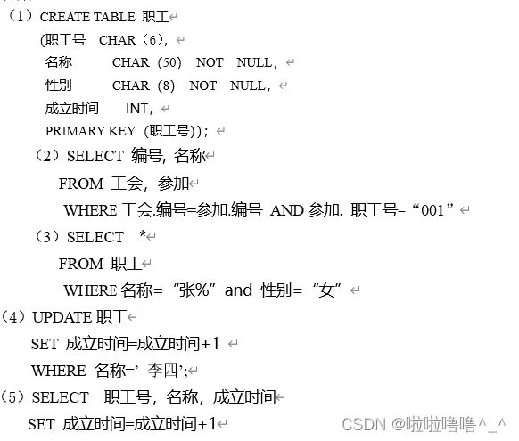
- TYUT太原理工大学2022数据库大题之分解关系模式
- View UI Plus 发布 1.1.0 版本,支持 SSR、支持 Nuxt、增加 TS 声明文件
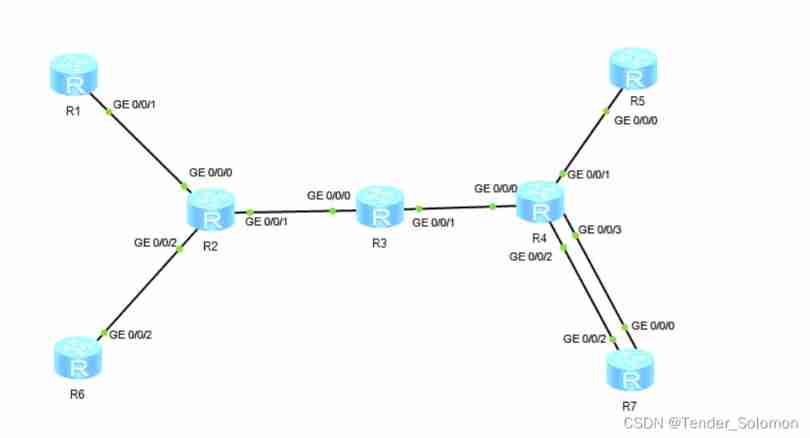
- IPv6 experiment
- Questions and answers of "Fundamentals of RF circuits" in the first semester of the 22nd academic year of Xi'an University of Electronic Science and technology
- 5. Function recursion exercise
猜你喜欢

Rich Shenzhen people and renting Shenzhen people
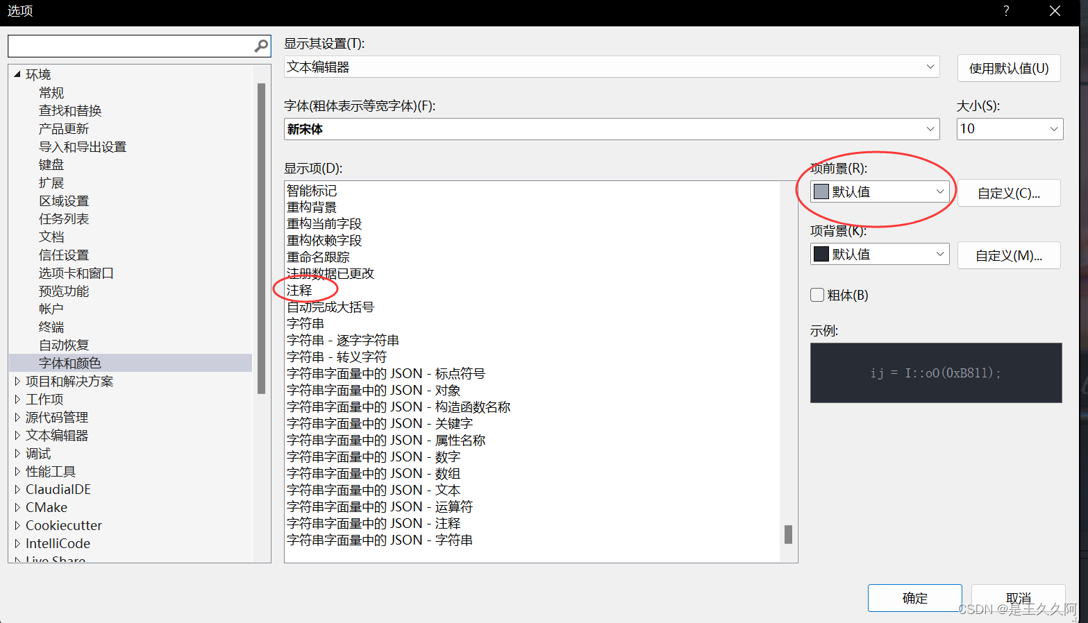
Change vs theme and set background picture
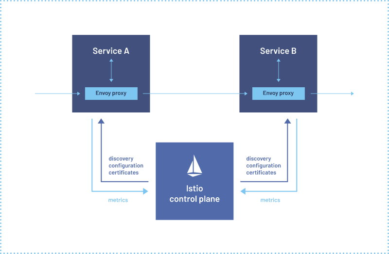
Alibaba cloud microservices (IV) service mesh overview and instance istio

Tyut Taiyuan University of technology 2022 "Mao Gai" must be recited
MPLS experiment
TYUT太原理工大学2022数据库大题之数据库操作
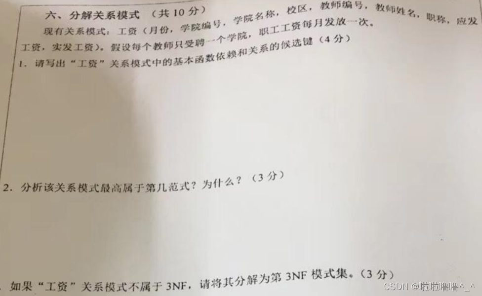
Decomposition relation model of the 2022 database of tyut Taiyuan University of Technology
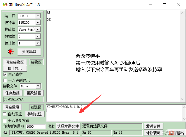
(超详细onenet TCP协议接入)arduino+esp8266-01s接入物联网平台,上传实时采集数据/TCP透传(以及lua脚本如何获取和编写)
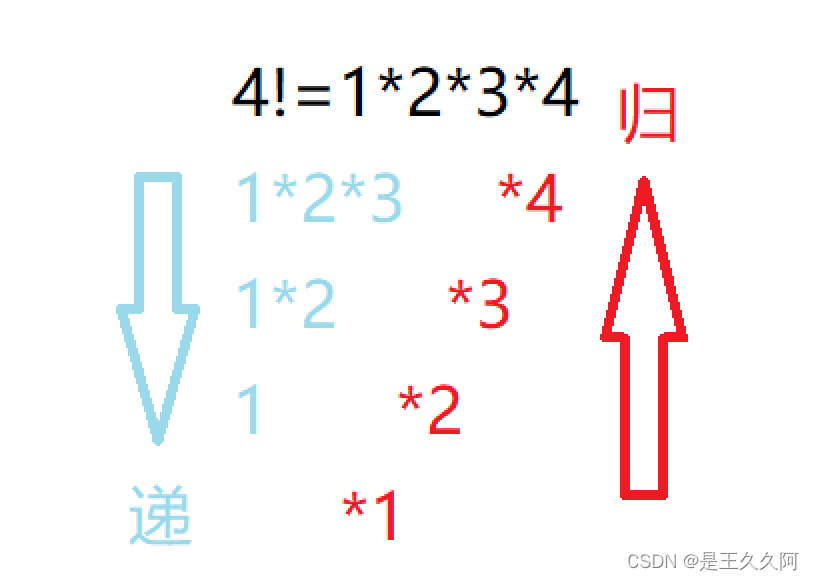
5. Function recursion exercise
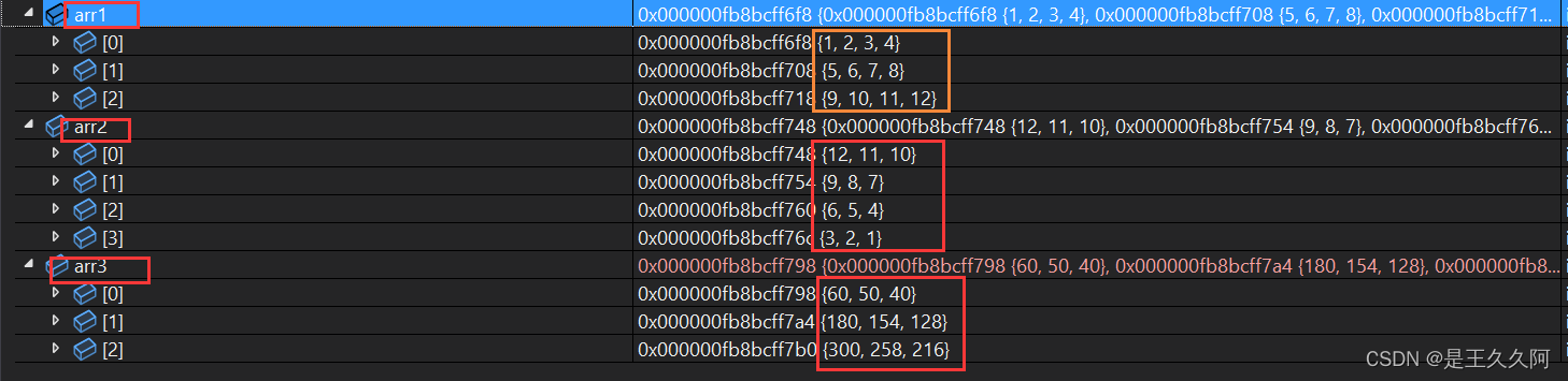
2. C language matrix multiplication
随机推荐
TYUT太原理工大学2022数据库大题之数据库操作
View UI plus releases version 1.1.0, supports SSR, supports nuxt, and adds TS declaration files
List set map queue deque stack
12 excel charts and arrays
The latest tank battle 2022 - Notes on the whole development -2
View UI Plus 发布 1.3.1 版本,增强 TypeScript 使用体验
4.二分查找
(super detailed II) detailed visualization of onenet data, how to plot with intercepted data flow
1.初识C语言(1)
[while your roommate plays games, let's see a problem]
Database operation of tyut Taiyuan University of technology 2022 database
TYUT太原理工大学2022数据库之关系代数小题
JS interview questions (I)
Application architecture of large live broadcast platform
Arduino+ds18b20 temperature sensor (buzzer alarm) +lcd1602 display (IIC drive)
4.30动态内存分配笔记
View UI Plus 发布 1.1.0 版本,支持 SSR、支持 Nuxt、增加 TS 声明文件
西安电子科技大学22学年上学期《射频电路基础》试题及答案
165. Compare version number - string
初识C语言(下)