当前位置:网站首页>Machine learning theory learning: perceptron
Machine learning theory learning: perceptron
2022-07-02 07:36:00 【wxplol】
List of articles
perceptron (Perceptron) It's a two class linear classification model , The input is the eigenvector of the instance , The output is the category of the instance , take +1 and -1. The perceptron corresponds to the input space ( The feature space ) The instance is divided into positive and negative separated hyperplanes , It's a discriminant model . Perceptron prediction is to use the learned perceptron model to classify new input instances , It is the basis of neural network and support vector machine . The following reference links are highly recommended , It's very detailed .
Refer to the connection :
machine learning —— perceptron
One 、 Perceptron model
Definition : Input x, Corresponding to the feature points in the input space , Output y={+1,-1} Represents the category of the instance , The functions input to output are as follows :
f ( x ) = s i g n ( w ∗ x + b ) f(x)=sign(w*x+b) f(x)=sign(w∗x+b)
It's called the perceptron .w、b Is the weight of the perceptron .
The perceptron is a linear classification model , It's a discriminant model . linear equation w*x+b=0 A hyperplane corresponding to the feature space S, This hyperplane divides the feature space into two parts , They are positive and negative .S Also called separating hyperplane , As shown in the figure below :

Two 、 Perceptron learning strategies
Suppose the training data is linearly separable , The learning goal of the perceptron is to find a separation hyperplane that can completely separate the positive and negative samples , That is, to be sure w,b, It is necessary to define a loss function and minimize the loss function .
The perceptron selects the misclassification point to the separation hyperplane S The total distance as a loss function . input space R n R^{n} Rn Any point in x o x_{o} xo The distance to the hyperplane :
1 ∣ ∣ w ∣ ∣ ∣ w ∗ x 0 + b ∣ \frac{1}{||w||}|w*x_{0}+b| ∣∣w∣∣1∣w∗x0+b∣
among ∣ ∣ w ∣ ∣ ||w|| ∣∣w∣∣ by w Of L2 norm .
【 Add 】
1、 The distance between a point and a line
Let the linear equation be Ax+By+C=0 , The last point is ( x 0 , y 0 ) (x_{0},y_{0}) (x0,y0), Then the distance is
d = A ∗ x 0 + B ∗ y 0 + C A 2 + B 2 d=\frac{A*x_{0}+B*y_{0}+C}{\sqrt{A^{2}+B^{2}}} d=A2+B2A∗x0+B∗y0+C
2、 Sample to hyperplane distanceSuppose the hyperplane is h=w⋅x+b, among w=(w0,w1,w2…wn), x=(x0,x1,x2…xn), Sample points x′ The distance to the hyperplane :
d = w ∗ x ′ + b ∣ ∣ d ∣ ∣ d=\frac{w*x^{'}+b}{||d||} d=∣∣d∣∣w∗x′+b
in addition , For misclassified classified data ( x i , y i ) (x_{i},y_{i}) (xi,yi) Come on , When w ∗ x i + b > 0 w*x_{i}+b>0 w∗xi+b>0 when , y i = − 1 y_{i}=-1 yi=−1; And when w ∗ x i + b < 0 w*x_{i}+b<0 w∗xi+b<0 when , y i = + 1 y_{i}=+1 yi=+1. therefore , Misclassification to S The distance to :
− 1 ∣ ∣ w ∣ ∣ y i ( w ∗ x i + b ) -\frac{1}{||w||}y_{i}(w*x_{i}+b) −∣∣w∣∣1yi(w∗xi+b)
Don't consider 1 ∣ ∣ w ∣ ∣ \frac{1}{||w||} ∣∣w∣∣1, The loss function of the perceptron is defined as :
L ( w , b ) = − ∑ y i ( w ∗ x i + b ) L(w,b)=-\sum y_{i}(w*x_{i}+b) L(w,b)=−∑yi(w∗xi+b)
3、 ... and 、 Perceptron learning algorithm
3.1、 The original form of Perceptron Algorithm
For a given data set T = ( x 1 , y 1 ) , . . . , ( x N , y N ) T={(x_{1},y_{1}),...,(x_{N},y_{N})} T=(x1,y1),...,(xN,yN) Find parameters w,b Minimize the loss function :
m i n L ( w , b ) = − ∑ y i ( w ∗ x i + b ) minL(w,b)=-\sum y_{i}(w*x_{i}+b) minL(w,b)=−∑yi(w∗xi+b)
Because we need to keep learning w,b, Therefore, we adopt the random gradient descent method to continuously optimize the objective function , ad locum , In the process of random gradient descent , Each time, only one misclassification point sample is used to reduce its gradient .
First , We solve the gradient , Respectively for w,bw,b Finding partial derivatives :
∇ w L ( w , b ) = ∂ ∂ w L ( w , b ) = − ∑ y i x i ∇ b L ( w , b ) = ∂ ∂ b L ( w , b ) = − ∑ y i ∇wL(w,b)=\frac{∂}{∂w}L(w,b)=−∑yixi\\ ∇bL(w,b)=\frac{∂}{∂b}L(w,b)=−∑yi ∇wL(w,b)=∂w∂L(w,b)=−∑yixi∇bL(w,b)=∂b∂L(w,b)=−∑yi
then , Randomly select a misclassification point pair w,bw,b updated : ( Synchronize updates )
w ← w + η y i x i b ← b + η y i w←w+ηyixi\\ b←b+ηyi w←w+ηyixib←b+ηyi
among ,η For learning rate , Through this iteration, the loss function L(w,b) Constantly decreasing , Until minimized .
Algorithm steps :
Input : T = ( x 1 , y 1 ) , . . . , ( x N , y N ) T={(x_{1},y_{1}),...,(x_{N},y_{N})} T=(x1,y1),...,(xN,yN), Learning rate η(0<η<=1)
Output :w,b; Perceptron model f ( x ) = s i g n ( w ∗ x + b ) f(x)=sign(w*x+b) f(x)=sign(w∗x+b)
- Select the initial value w 0 , b 0 w_{0},b_{0} w0,b0
- Select data ( x i , y i ) (x_{i},y_{i}) (xi,yi)
- If y i ( w ∗ x i + b ) < = 0 y_{i}(w*x_{i}+b)<=0 yi(w∗xi+b)<=0
w ← w + η y i x i b ← b + η y i w←w+ηyixi\\ b←b+ηyi w←w+ηyixib←b+ηyi
- Transferred to (2), There are no misclassification points until the training set
According to the algorithm, we can see , Perceptron mainly uses misclassification points to learn , Through adjustment w,b Value , Move the separation hyperplane to the misclassification point , Reduce the distance from the separation point to the plane , Until the hyperplane crosses the point so that it is correctly classified .
3.2、 Dual form of Perceptron Algorithm
We know the general form of weight update :
w ← w + η y i x i b ← b + η y i w←w+ηyixi\\ b←b+ηyi w←w+ηyixib←b+ηyi
But after many iterations , We need to update many times w、b The weight , This calculation is relatively large . Is there a way to calculate the weight without so many times ? Yes , That is the dual form of Perceptron Algorithm . Specifically, how to lead out can ? We know what happened n After modification , The parameter changes are as follows :
w = ∑ i a i y i x i b = ∑ i a i y i w=\sum_{i} a_{i}y_{i}x_{i} \\ b=\sum_{i} a_{i}y_{i} w=i∑aiyixib=i∑aiyi
among a i a_{i} ai It is a misclassification point ( x i , y i ) (x_{i},y_{i}) (xi,yi) Number of updates required
So we can learn from w,b Become the number of learning misclassification a i a_{i} ai, And in the dual form Gram Matrix to store the inner product , It can improve the operation speed , In contrast to the original form , Every time the parameters change , All matrix calculations need to be calculated , This leads to a much larger amount of computation than the dual form , This is the efficiency of the dual form . here Gram The matrix is equivalent to ∑ i y i x i \sum_{i}y_{i}x_{i} ∑iyixi.Gram The definition of a matrix is as follows :
G = [ x 1 x 1 . . . x 1 x N x 2 x 1 . . . x 2 x N . . . . . . . . . x N x 1 . . . x N x N ] G=\left[ \begin{matrix} x_{1}x_{1} & ... & x_{1}x_{N}\\ x_{2}x_{1} & ... & x_{2}x_{N}\\ ... & ... & ...\\ x_{N}x_{1} & ... & x_{N}x_{N} \end{matrix} \right] G=⎣⎢⎢⎡x1x1x2x1...xNx1............x1xNx2xN...xNxN⎦⎥⎥⎤
Algorithm steps :
Input : T = ( x 1 , y 1 ) , . . . , ( x N , y N ) T={(x_{1},y_{1}),...,(x_{N},y_{N})} T=(x1,y1),...,(xN,yN), Learning rate η(0<η<=1)
Output :a,b; Perceptron model f ( x ) = s i g n ( ∑ j a j y i x j ∗ x i + b ) f(x)=sign(\sum_{j}a_{j}y_{i}x_{j}*x_{i}+b) f(x)=sign(∑jajyixj∗xi+b)
- Assign initial value to a0,b0 .
- Select data points (xi,yi).
- Judge whether the data point is the misclassification point of the current model , That is, judge if y i ( ∑ j a j y j x j ∗ x i + b ) < = 0 y_{i}(\sum_{j}a_{j}y_{j}x_{j}*x_{i}+b)<=0 yi(∑jajyjxj∗xi+b)<=0 Update
a i = a i + η b = b + η y i a_{i}=a_{i}+η \\ b=b+ηy_{i} ai=ai+ηb=b+ηyi
- go to (2), Until there are no misclassification points in the training set
In order to reduce the amount of calculation , We can calculate the inner product in the formula in advance , obtain Gram matrix .
Refer to the connection :
Introduction to machine learning 《 Statistical learning method 》 Take notes —— perceptron
边栏推荐
- Drawing mechanism of view (3)
- Interpretation of ernie1.0 and ernie2.0 papers
- A summary of a middle-aged programmer's study of modern Chinese history
- [medical] participants to medical ontologies: Content Selection for Clinical Abstract Summarization
- Get the uppercase initials of Chinese Pinyin in PHP
- Spark SQL task performance optimization (basic)
- allennlp 中的TypeError: Object of type Tensor is not JSON serializable错误
- JSP intelligent community property management system
- PPT的技巧
- Alpha Beta Pruning in Adversarial Search
猜你喜欢
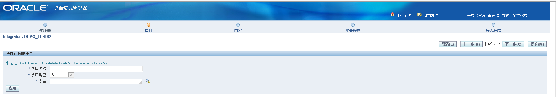
Oracle EBS ADI development steps

Faster-ILOD、maskrcnn_benchmark训练自己的voc数据集及问题汇总
![[paper introduction] r-drop: regulated dropout for neural networks](/img/09/4755e094b789b560c6b10323ebd5c1.png)
[paper introduction] r-drop: regulated dropout for neural networks
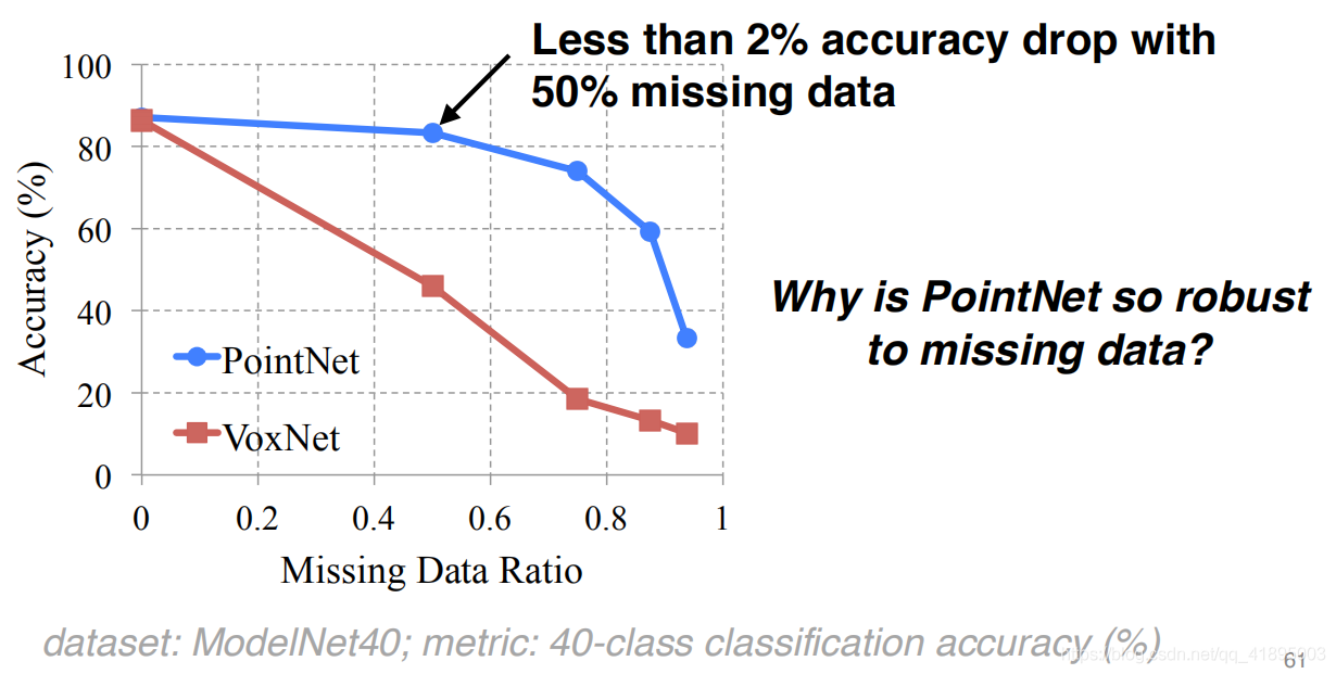
PointNet理解(PointNet实现第4步)

Record of problems in the construction process of IOD and detectron2

Error in running test pyspark in idea2020
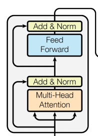
【深度学习系列(八)】:Transoform原理及实战之原理篇
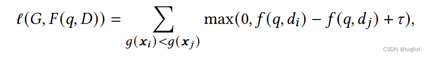
【Ranking】Pre-trained Language Model based Ranking in Baidu Search
Point cloud data understanding (step 3 of pointnet Implementation)
【论文介绍】R-Drop: Regularized Dropout for Neural Networks
随机推荐
【信息检索导论】第六章 词项权重及向量空间模型
矩阵的Jordan分解实例
Conda 创建,复制,分享虚拟环境
Oracle 11g uses ords+pljson to implement JSON_ Table effect
Calculate the difference in days, months, and years between two dates in PHP
[introduction to information retrieval] Chapter 1 Boolean retrieval
Mmdetection installation problem
传统目标检测笔记1__ Viola Jones
Yaml file of ingress controller 0.47.0
Implementation of yolov5 single image detection based on onnxruntime
How do vision transformer work?【论文解读】
Using MATLAB to realize: Jacobi, Gauss Seidel iteration
[introduction to information retrieval] Chapter 7 scoring calculation in search system
解决万恶的open failed: ENOENT (No such file or directory)/(Operation not permitted)
基于pytorch的YOLOv5单张图片检测实现
【信息检索导论】第二章 词项词典与倒排记录表
SSM laboratory equipment management
Two dimensional array de duplication in PHP
MMDetection模型微调
《Handwritten Mathematical Expression Recognition with Bidirectionally Trained Transformer》论文翻译