Mikolov T , Chen K , Corrado G , et al. Efficient Estimation of Word Representations in Vector Space[J]. Computer ence, 2013.
Source code :https://github.com/danielfrg/word2vec
The purpose of the article
The purpose of this paper is to propose learning high quality word vectors (word2vec) Methods , These methods are mainly used in data sets of one billion or millions of words . Therefore, the author proposes two novel models (CBOW,Skip-gram) To compute the continuous vector representation , The quality of expression is measured by the similarity of words , Compare the results with the previous best performance neural network model .
The author attempts to maximize vector operations with a new model structure , And keep the linear rules between words . At the same time, it discusses how the training time and accuracy depend on the dimension of the word vector and the amount of training data .
Conclusion
- The new model reduces the computational complexity , Improved accuracy ( from 160 Learning high quality word vectors in 100 million word data sets )
- These vectors provide state-of-the-art performance for metrics syntax and semantics on the test set .
background
some NLP Systems and tasks use words as atomic units , There is no similarity between words , It is expressed as a subscript of a dictionary , There are several advantages to this approach : Simple , Robust , A simple model trained on a large data set is better than a complex model trained on a small data set . The most popular one is for statistical language models N Metamodel , today , It can train almost all data n Metamodel .
These simple techniques have limitations on many tasks . So simply improving these basic technologies doesn't make a significant difference , We have to focus on more advanced technology .
Model Architectures
Many researchers have proposed many different types of models before , for example LSA and LDA. In this paper , The author mainly studies the word distributed representation of neural network learning .
To compare the computational complexity of different models , The following model training complexity is proposed :
- E: Number of training iterations
- T: The number of words in the training set
- Q:Q Further defined by each model , As follows .
Feedforward Neural Net Language Model(NNLM)
structure :
- Input Layer: Use one-hot Coded N Words before ,V Is the size of the glossary
- Projection Layer: Dimension is \(N×D\), Using a shared projection matrix
- Hidden Layer:H Represents the number of hidden layer nodes
- Output Layer:V Represents the number of output nodes
The computational complexity formula for each sample is as follows :
- \(N×D\): Input the number of weights from the layer to the projection ,N It's the length of the context ,D It is the real number of each word that represents the dimension
- \(N×D×H\): The number of weights from the projection layer to the hidden layer
- \(H×V\): The number of weights from hidden layer to output layer
The most important thing was \(H×V\), But the author proposes to use hierarchical softmax Or avoid using a regularized model to deal with it . Which uses Huffman binary Trees are used to represent words , The number of output units to be evaluated has decreased \(log_2(V)\). therefore , Most of the computational complexity comes from \(N×D×H\) term .
Recurrent Neural Net Language Model (RNNLM)
The recurrent neural network based on language model mainly overcomes feedforward NNLM The shortcomings of , For example, you need to determine the length of the text .RNN Can represent more complex models .
structure :
- Input Layer: Words mean D And hidden layer H They have the same dimensions
- Hidden Layer:H Represents the number of hidden layer nodes
- Output Layer:V Represents the number of output nodes
The characteristic of this model is that there is a circular matrix connecting hidden layers , Connection with time delay , This allows for the formation of long-term memory , Past information can be represented by hidden states , The update of the hidden state is determined by the state of the hidden layer of the current input and the previous input
The computational complexity formula for each sample is as follows :
- \(H×H\): Enter the number of weights from the layer to the hidden layer
- \(H×V\): The number of hidden layers to output layers
Again , Use hierarchical softmax You can put \(H×V\) Item is effectively reduced to \(H×log_2(V)\) term . So most of the complexity comes from \(H×H\) term .
Parallel Training of Neural Networks
The author in Google A large distributed framework for DistBelief Several models are implemented on , This framework allows us to run different copies of the same model in parallel , Each copy updates the parameters through a central server that stores all the parameters . For this kind of parallel training , Author use mini-batch Asynchronous gradient descent and one called Adagrad Adaptive learning rate of . In this frame , Usually use one hundred or more copies , Each replica is used on one machine in one data center CPU The core .
The proposed model
The author proposes two new models (New Log-linear Models) To learn the expression of words , The advantage of the new model is that it reduces the computational complexity . It is found that a large amount of computational complexity mainly comes from the nonlinear hidden layer in the model .
The two new models have similar model structures , There are Input layer 、Projection Layer and the Output layer .
Continuous Bag-of-Words Model
The input is the word vector corresponding to the context sensitive word of a feature word , And the output is the word vector of this particular word .
and NNLM Compared with the removal of nonlinear hidden layer , And the projection layer is shared with all the words ( It's not just the sharing of projective matrices ). therefore , All the words are projected onto a D On the vector of dimension ( Add and average ).

The computational complexity is :
Continuous Skip-gram Model
The input is a word vector for a particular word , The output is the context word vector corresponding to a specific word .
Use the current word as input , Input to a projection layer , Then it predicts the context of the current word .
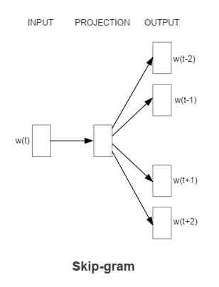
The computational complexity is :
- C: The maximum distance between words
Comments
For the detailed analysis of these two models, please refer to this paper :Rong X . word2vec Parameter Learning Explained[J]. Computer ence, 2014.