当前位置:网站首页>1. Linear regression
1. Linear regression
2022-07-08 01:02:00 【booze-J】
The code running platform is jupyter-notebook, Code blocks in the article , According to jupyter-notebook Written in the order of division in , Run article code , Glue directly into jupyter-notebook that will do .
1. Import third-party library
import keras
import numpy as np
import matplotlib.pyplot as plt
# Sequential  Sequential model
from keras.models import Sequential
# Dense  Fully connected layer
from keras.layers import Dense
2. Randomly generate data sets
#  Use numpy Generate 100 A random point
x_data = np.random.rand(100)
#  Noise shape and x_data The shape of is the same
noise = np.random.normal(0,0.01,x_data.shape)
#  Set up w=0.1 b=0.2
y_data = x_data*0.1+0.2+noise
# y_data_no_noisy = x_data*0.1+0.2
#  Show random points
plt.scatter(x_data,y_data)
# plt.scatter(x_data,y_data_no_noisy)
Running effect :
This is the case of adding noise y_data = x_data*0.1+0.2+noise: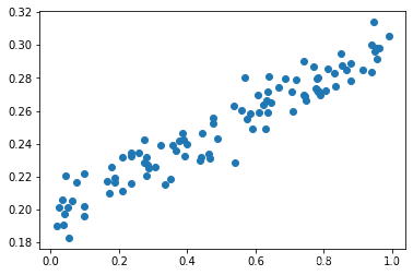
Without adding noise y_data_no_noisy = x_data*0.1+0.2(w=0.1,b=0.2):
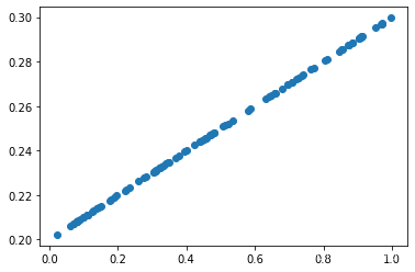
Linear regression is based on the scatter plot with added noise , Fit a straight line that is similar to the scatter diagram without adding noise .
3. Linear regression
# Build a sequential model
model = Sequential()
# Add a full connection layer to the model stay jupyter-notebook in , Press shift+tab Parameters can be displayed
model.add(Dense(units=1,input_dim=1))
# sgd:Stochastic gradient descent , Random gradient descent method
# mse:Mean Squared Error , Mean square error
model.compile(optimizer='sgd',loss='mse')
# Training 3001 Lots
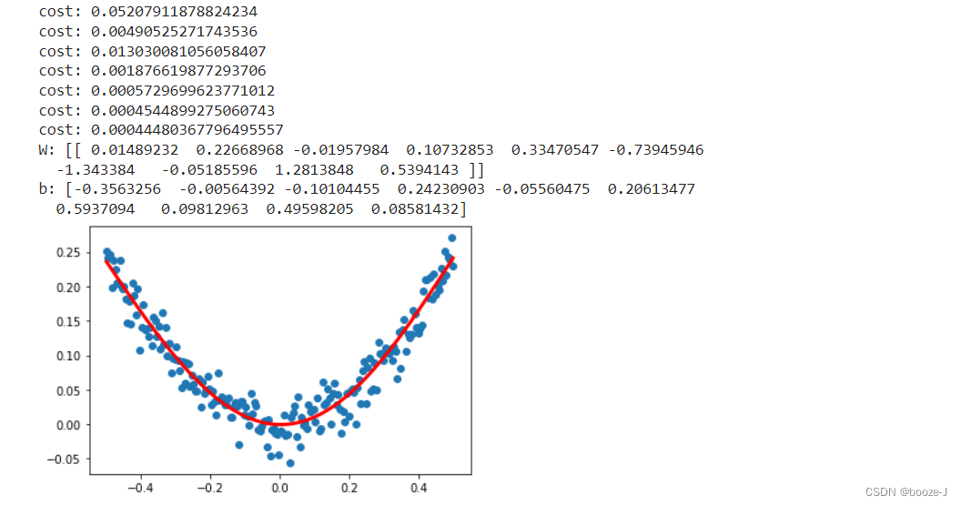
for step in range(3001):
# One batch at a time The loss of
cost = model.train_on_batch(x_data,y_data)
# Every time 500 individual batch Print once cost
if step%500==0:
print("cost:",cost)
# Print weights and batch values
W,b = model.layers[0].get_weights()
print("W:",W)
print("b:",b)
# x_data Input the predicted value in the network
y_pred = model.predict(x_data)
# Show random points
plt.scatter(x_data,y_data)
# Show forecast results
plt.plot(x_data,y_pred,"r-",lw=3)
plt.show()
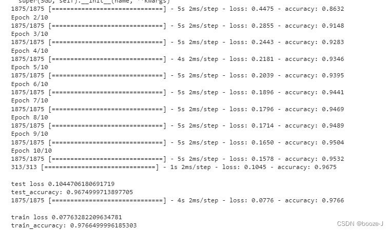
Running effect :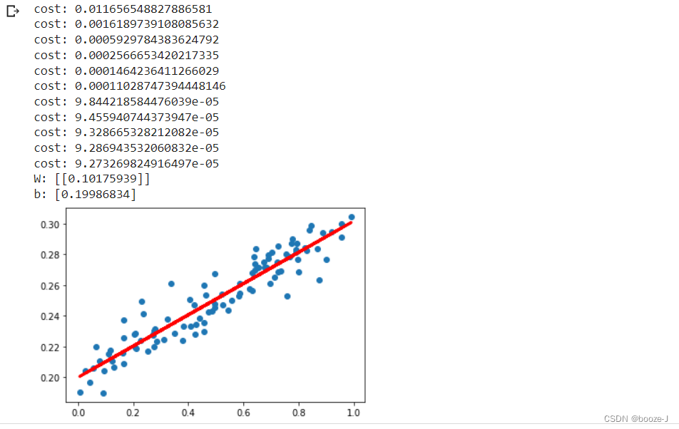
You can see the prediction w and b Are very close to what we set w and b.
Be careful
- stay jupyter-notebook in , Press shift+tab Parameters can be displayed
- train_on_batch Use
- compile Use
边栏推荐
- Swift get URL parameters
- 手写一个模拟的ReentrantLock
- Cve-2022-28346: Django SQL injection vulnerability
- Is it safe to speculate in stocks on mobile phones?
- 8道经典C语言指针笔试题解析
- [Yugong series] go teaching course 006 in July 2022 - automatic derivation of types and input and output
- Su embedded training - Day8
- What has happened from server to cloud hosting?
- Langchao Yunxi distributed database tracing (II) -- source code analysis
- Basic mode of service mesh
猜你喜欢


随机推荐
New library online | information data of Chinese journalists
Leetcode brush questions
ReentrantLock 公平锁源码 第0篇
Introduction to paddle - using lenet to realize image classification method II in MNIST
Thinkphp内核工单系统源码商业开源版 多用户+多客服+短信+邮件通知
130. Zones environnantes
1293_ Implementation analysis of xtask resumeall() interface in FreeRTOS
接口测试进阶接口脚本使用—apipost(预/后执行脚本)
Semantic segmentation model base segmentation_ models_ Detailed introduction to pytorch
【笔记】常见组合滤波电路
Cancel the down arrow of the default style of select and set the default word of select
Reentrantlock fair lock source code Chapter 0
4.交叉熵
QT establish signal slots between different classes and transfer parameters
手写一个模拟的ReentrantLock
133. 克隆图
Tapdata 的 2.0 版 ,开源的 Live Data Platform 现已发布
Interface test advanced interface script use - apipost (pre / post execution script)
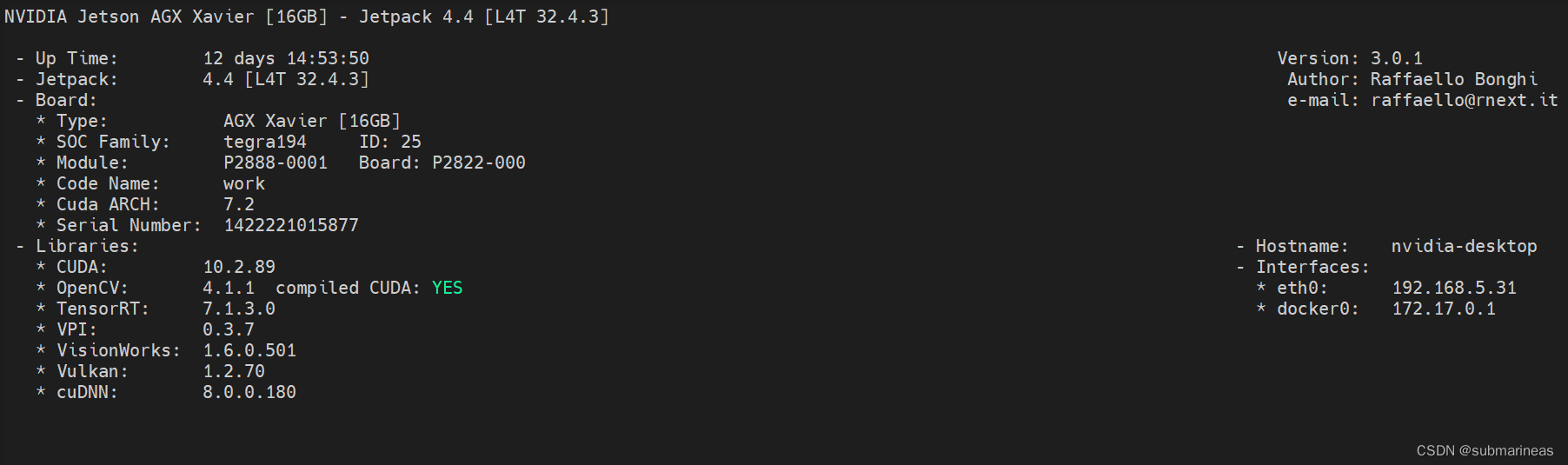
NVIDIA Jetson test installation yolox process record
Hotel