当前位置:网站首页>Numpy quick start (III) -- array advanced operation
Numpy quick start (III) -- array advanced operation
2022-07-03 10:40:00 【serity】
Catalog
One 、 Change the shape of the array
| function | effect |
|---|---|
| np.reshape(a, newshape) | a yes Array ,newshape yes Integer tuple ; return newshape Array of shapes |
| np.ravel(a) | It's a fair show One dimensional array ; Equivalent to np.reshape(a, -1) |
| np.flatten(a) | Effect and ravel equally , but More recommended Use flatten |
1.1 np.reshape()
A = np.arange(6).reshape((2, 3))
print(A)
# [[0 1 2]
# [3 4 5]]
In fact, the parentheses of the meta Group It can be omitted , That is, we can use reshape:
A = np.arange(6).reshape(2, 3)
newshape One of them One The component can be -1,reshape It will automatically calculate according to other components :
A = np.arange(6).reshape(2, -1)
print(A)
# [[0 1 2]
# [3 4 5]]
if newshape = -1, that reshape Will flatten it to One dimensional array :
A = np.arange(6).reshape(6).reshape(-1)
print(A)
# [0 1 2 3 4 5]
1.2 np.ravel()
A = np.arange(8).reshape(2, 2, 2).ravel()
print(A)
# [0 1 2 3 4 5 6 7]
1.3 np.flatten()
A = np.arange(8).reshape(2, 2, 2).flatten()
print(A)
# [0 1 2 3 4 5 6 7]
It can be seen that flatten The effect and ravel equally , Which one is better to use ?
Just say the answer : Use flatten Better , See Blog .
Two 、( class ) Transpose operation
| function | effect |
|---|---|
| ndarray.T | Transposition An array , I.e. reverse shape |
| np.swapaxes(a, axis1, axis2) | In exchange for Two axes of the array |
| np.moveaxis(a, s, d) | s and d yes Integers or Integer list ; Index is s The axis of moves to the index d It's about |
2.1 ndarray.T
A = np.arange(6).reshape(2, 3)
print(A)
print(A.T)
# [[0 1 2]
# [3 4 5]]
# [[0 3]
# [1 4]
# [2 5]]
But should pay attention to ,ndarray.T Cannot transpose a one-dimensional array :
A = np.arange(6)
print(A)
print(A.T)
# [0 1 2 3 4 5]
# [0 1 2 3 4 5]
How do we transpose a one-dimensional array ? There are several ways :
Method 1 : First convert to a two-dimensional array
take ndarray Become a two-dimensional array and transpose :
A = np.arange(4)
A = np.array([A])
print(A.T)
# [[0]
# [1]
# [2]
# [3]]
You can also use it np.transpose(), It is associated with ndarray.T Equivalent :
A = np.arange(4)
print(np.transpose([A]))
# [[0]
# [1]
# [2]
# [3]]
Method 2 : Use reshape function
A = np.arange(4)
A = A.reshape(len(A), -1)  #  The second parameter is changed to 1 It's fine too
print(A)
# [[0]
# [1]
# [2]
# [3]]
Method 3 : Use newaxis
We mentioned in the first article of this series np.newaxis, Here we will further explain its usage .
newaxis The essence is None:
print(np.newaxis == None)
# True
As its name suggests , take newaxis and Using slices together, you can add a New dimensions ( Axis ), It can change a one-dimensional array into a two-dimensional array , Change a two-dimensional array into a three-dimensional array , You can also directly change a one-dimensional array into a three-dimensional array .
Ingenious notes : newaxis On which axis , Then the length of the result along the axis is 1
It may not be easy to understand , Here are some examples . hypothesis A Is a length of 3 One dimensional array of , be :
A[np.newaxis, :]: newaxis Located on the first axis , The result is 1 × 3 1\times 3 1×3 Array of .A[:, np.newaxis]: newaxis Located on the second axis , The result is 3 × 1 3\times1 3×1 Array of .A[:, np.newaxis, np.newaxis]: newaxis Located on the second and third axes , The result is 3 × 1 × 1 3\times1\times1 3×1×1 Array of .
Let's give a few more examples and combine shape Methods to further illustrate newaxis The effect of .
First create a 3 × 4 3\times4 3×4 Array of :
A = np.arange(12).reshape(3, 4)
print(A.shape)
# (3, 4)
And then use newaxis Add a new axis :
print(A[:, :, np.newaxis].shape)
print(A[:, np.newaxis, :].shape)
print(A[np.newaxis, :, :].shape)
print(A[np.newaxis, np.newaxis, :, :].shape)
# (3, 4, 1)
# (3, 1, 4)
# (1, 3, 4)
# (1, 1, 3, 4)
After reading these examples , Believe that you are newaxis There is already a basic cognition , How to transpose a dimensional array is no longer difficult .
Because the transposed one-dimensional array must be shaped like a × 1 a\times 1 a×1 The shape of the , therefore newaxis It must be on the second axis , So you just need to A[:, np.newaxis] You can transpose :
A = np.arange(4)
print(A[:, np.newaxis])
# [[0]
# [1]
# [2]
# [3]]
2.2 np.swapaxes()
A = np.zeros((3, 4, 5))
print(A.shape)
# (3, 4, 5)
print(np.swapaxes(A, 0, 1).shape)
print(np.swapaxes(A, 0, 2).shape)
print(np.swapaxes(A, 1, 2).shape)
# (4, 3, 5)
# (5, 4, 3)
# (3, 5, 4)
2.3 np.moveaxis()
s and d When all are integers :
A = np.zeros((3, 4, 5))
print(np.moveaxis(A, 0, 2).shape)
print(np.moveaxis(A, 0, -1).shape)
print(np.moveaxis(A, -1, -2).shape)
# (4, 5, 3)
# (4, 5, 3)
# (3, 5, 4)
s and d When both are integer lists :
A = np.zeros((3, 4, 5))
print(np.moveaxis(A, [0, 1], [1, 2]).shape)
print(np.moveaxis(A, [0, 1], [0, 2]).shape)
print(np.moveaxis(A, [1, 0], [0, 2]).shape)
# (5, 3, 4)
# (3, 5, 4)
# (4, 5, 3)
3、 ... and 、 Merge array
| function | effect |
|---|---|
| np.concatenate((a1, a2, …), axis=0) | a1, a2 Is such as Array ,axis control Direction of connection ; Used to convert multiple arrays come together , When axis by None when , Before connecting Flatten Each array to be connected |
| np.stack(arrays, axis=0) | arrays Is composed of arrays List or tuple ; Along the axis Direction The stack These arrays |
| np.block(arrays) | Put several arrays Combine Together to form a new array ; Often used to build Block matrix |
| np.vstack((a1, a2, …)) | vertical Stacked array |
| np.hstack((a1, a2, …)) | level Stacked array |
3.1 np.concatenate()
a = np.array([[1, 2], [3, 4]])
b = np.array([[5, 6]])
print(np.concatenate((a, b), axis=0))
# [[1 2]
# [3 4]
# [5 6]]
print(np.concatenate((a, b.T), axis=1))
# [[1 2 5]
# [3 4 6]]
print(np.concatenate((a, b), axis=None))
# [1 2 3 4 5 6]
To connect two one-dimensional arrays , It only needs :
a = np.array([1, 2])
b = np.array([3, 4])
print(np.concatenate((a, b)))
# [1 2 3 4]
3.2 np.stack()
a = np.array([1, 2, 3])
b = np.array([4, 5, 6])
print(np.stack((a, b)))
# [[1 2 3]
# [4 5 6]]
print(np.stack((a, b), axis=1))
# [[1 4]
# [2 5]
# [3 6]]
arrays = [np.zeros((2, 3)) for _ in range(4)]
print(np.stack(arrays, axis=0).shape)
print(np.stack(arrays, axis=1).shape)
print(np.stack(arrays, axis=2).shape)
# (4, 2, 3)
# (2, 4, 3)
# (2, 3, 4)
be aware axis=2 It's actually the last axis , We can also use axis=-1 To replace it , The effect is the same , Other shafts can also be pushed :
print(np.stack(arrays, axis=-3).shape)
print(np.stack(arrays, axis=-2).shape)
print(np.stack(arrays, axis=-1).shape)
# (4, 2, 3)
# (2, 4, 3)
# (2, 3, 4)
3.3 np.block()
A = np.eye(2) * 2
B = np.eye(3) * 3
C = np.block([
		  [A,               np.zeros((2, 3))],
          [np.ones((3, 2)), B               ]
    ])
print(C)
# [[2. 0. 0. 0. 0.]
# [0. 2. 0. 0. 0.]
# [1. 1. 3. 0. 0.]
# [1. 1. 0. 3. 0.]
# [1. 1. 0. 0. 3.]]
3.3 np.vstack()
a = np.array([1, 2, 3])
b = np.array([4, 5, 6])
print(np.vstack((a, b)))
# [[1 2 3]
# [4 5 6]]
A more vivid explanation : Because it is stacked vertically , So the B B B Put it in A A A below
A = [ 1 , 2 , 3 ] , B = [ 4 , 5 , 6 ] A=[1, 2, 3],\quad B=[4,5,6] A=[1,2,3],B=[4,5,6]
a = np.array([[1], [2], [3]])
b = np.array([[4], [5], [6]])
print(np.vstack((a, b)))
# [[1]
# [2]
# [3]
# [4]
# [5]
# [6]]
In the same way B B B Put it in A A A below
A = [ 1 2 3 ] , B = [ 4 5 6 ] A=\begin{bmatrix} 1 \\ 2\\ 3 \\ \end{bmatrix} ,\quad B=\begin{bmatrix} 4 \\ 5\\ 6 \\ \end{bmatrix} A=⎣⎡123⎦⎤,B=⎣⎡456⎦⎤
3.4 np.hstack()
a = np.array([1, 2, 3])
b = np.array([4, 5, 6])
print(np.hstack((a, b)))
# [1 2 3 4 5 6]
A more vivid explanation : Because it is stacked horizontally , So the B B B Put it in A A A On the right
A = [ 1 , 2 , 3 ] , B = [ 4 , 5 , 6 ] A=[1, 2, 3],\quad B=[4,5,6] A=[1,2,3],B=[4,5,6]
a = np.array([[1], [2], [3]])
b = np.array([[4], [5], [6]])
print(np.hstack((a, b)))
# [[1 4]
# [2 5]
# [3 6]]
In the same way B B B Put it in A A A On the right
A = [ 1 2 3 ] , B = [ 4 5 6 ] A=\begin{bmatrix} 1 \\ 2\\ 3 \\ \end{bmatrix} ,\quad B=\begin{bmatrix} 4 \\ 5\\ 6 \\ \end{bmatrix} A=⎣⎡123⎦⎤,B=⎣⎡456⎦⎤
Four 、 Partition array
| function | effect |
|---|---|
| np.split(a, indices/sections) | Will array a Divide it into sub arrays and return it as a list ;sections Is the number of subarrays ,indices Is an index list ; It can be divided by quantity or by index position |
| np.array_split(a, indices/sections) | And split The only difference is , When selecting quantity division , No need The shape of each subarray is required to be the same |
| np.vsplit(a, indices/sections) | vertical Partition array |
| np.hsplit(a, indices/sections) | level Partition array |
4.1 np.split()
Divide by quantity , Of each subarray The same shape :
a = np.arange(9)
print(np.split(a, 3))
# [array([0, 1, 2]), array([3, 4, 5]), array([6, 7, 8])]
print(np.split(a, 4))
# ValueError: array split does not result in an equal division
The reason for the error is that you cannot set the length to 9 Array quartering .
Of course, we can also divide by index :
a = np.arange(9)
print(np.split(a, [2, 5]))
# [array([0, 1]), array([2, 3, 4]), array([5, 6, 7, 8])]
print(np.split(a, [1, 3, 5, 7]))
# [array([0]), array([1, 2]), array([3, 4]), array([5, 6]), array([7, 8])]
4.2 np.array_split()
a = np.arange(9)
print(np.array_split(a, 4))
# [array([0, 1, 2]), array([3, 4]), array([5, 6]), array([7, 8])]
4.3 np.vsplit()
By quantity :
a = np.arange(16).reshape(4, 4)
print(np.vsplit(a, 2))
# [array([[0, 1, 2, 3],
# [4, 5, 6, 7]]), array([[ 8, 9, 10, 11],
# [12, 13, 14, 15]])]
By index :
a = np.arange(16).reshape(4, 4)
print(np.vsplit(a, [1, 2]))
# [array([[0, 1, 2, 3]]), array([[4, 5, 6, 7]]), array([[ 8, 9, 10, 11],
# [12, 13, 14, 15]])]
When the dimension of the array is greater than or equal to 3 when , The division direction is still along The first axis ( That's ok ):
a = np.arange(8).reshape(2, 2, 2)
print(np.vsplit(a, 2))
# [array([[[0, 1],
# [2, 3]]]), array([[[4, 5],
# [6, 7]]])]
4.4 np.hsplit()
By quantity :
a = np.arange(16).reshape(4, 4)
print(np.hsplit(a, 2))
# [array([[ 0, 1],
# [ 4, 5],
# [ 8, 9],
# [12, 13]]), array([[ 2, 3],
# [ 6, 7],
# [10, 11],
 # [14, 15]])]
By index :
a = np.arange(16).reshape(4, 4)
print(np.hsplit(a, [1, 2]))
# [array([[ 0],
# [ 4],
# [ 8],
# [12]]), array([[ 1],
# [ 5],
# [ 9],
# [13]]), array([[ 2, 3],
# [ 6, 7],
# [10, 11],
# [14, 15]])]
When the dimension of the array is greater than or equal to 3 when , The division direction is still along The second axis ( Column ):
a = np.arange(8).reshape(2, 2, 2)
print(np.hsplit(a, 2))
# [array([[[0, 1]],

# [[4, 5]]]), array([[[2, 3]],

# [[6, 7]]])]
5、 ... and 、 Inversion array
| function | effect |
|---|---|
| np.flip(a, axis=None) | Along the axis Direction reversal array a;axis by Integers or Integer tuple ; When axis by None, Will move the array along All shafts Reverse . When axis When is a tuple , Will put the array along the tuple Shaft mentioned Reverse |
| np.fliplr(a) | Along the The second axis ( Column direction ) Reverse |
| np.flipud(a) | Along the The first axis ( Line direction ) Reverse |
5.1 np.flip()
Consider a one-dimensional array first :
a = np.arange(6)
print(np.flip(a))
# [5 4 3 2 1 0]
For two dimensional arrays :
A = np.arange(8).reshape(2, 2, 2)
print(A)
# [[[0 1]
# [2 3]]
#
# [[4 5]
# [6 7]]]
print(np.flip(A, axis=0))
# [[[4 5]
# [6 7]]
#
# [[0 1]
# [2 3]]]
print(np.flip(A, axis=1))
# [[[2 3]
# [0 1]]
#
# [[6 7]
# [4 5]]]
print(np.flip(A, axis=2))
# [[[1 0]
# [3 2]]
#
# [[5 4]
# [7 6]]]
print(np.flip(A))
# [[[7 6]
# [5 4]]
#
# [[3 2]
# [1 0]]]
print(np.flip(A, axis=(0, 2)))
# [[[5 4]
# [7 6]]
#
# [[1 0]
# [3 2]]]
5.2 np.fliplr()
A = np.diag([1, 2, 3])
print(np.fliplr(A))
# [[0 0 1]
# [0 2 0]
# [3 0 0]]
5.3 np.flipud()
A = np.diag([1, 2, 3])
print(np.flipud(A))
# [[0 0 3]
# [0 2 0]
# [1 0 0]]
Now? , We can flip() Function to make a summary :
flip(a, 0)Equivalent toflipud(a)flip(a, 1)Equivalent tofliplr(a)flip(a, n)Equivalent toa[..., ::-1, ...], among::-1The index of isnflip(a)Equivalent toa[::-1, ::-1, ..., ::-1], All of them are::-1flip(a, (0, 1))Equivalent toa[::-1, ::-1, ...], Only index0and1Place is::-1
边栏推荐
猜你喜欢
Hands on deep learning pytorch version exercise solution-3.3 simple implementation of linear regression
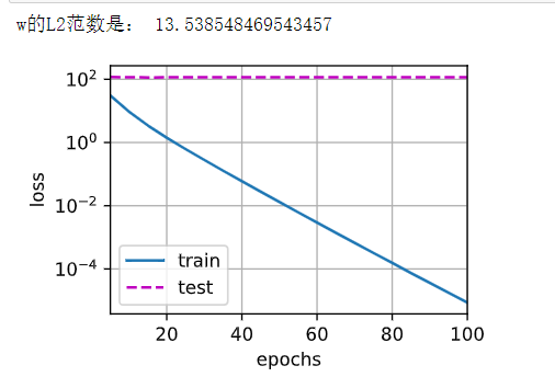
Weight decay (pytorch)

Out of the box high color background system

Knowledge map enhancement recommendation based on joint non sampling learning

8、 Transaction control language of MySQL
七、MySQL之数据定义语言(二)

Ut2016 learning notes

安装yolov3(Anaconda)
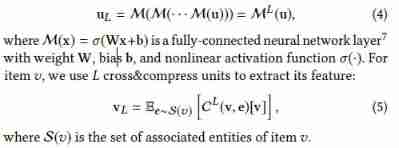
Multi-Task Feature Learning for Knowledge Graph Enhanced Recommendation

Convolutional neural network (CNN) learning notes (own understanding + own code) - deep learning
随机推荐
Mysql5.7 installation and configuration tutorial (Graphic ultra detailed version)
实战篇:Oracle 数据库标准版(SE)转换为企业版(EE)
Leetcode刷题---44
ThreadLocal原理及使用场景
Are there any other high imitation projects
Leetcode skimming ---75
Linear regression of introduction to deep learning (pytorch)
熵值法求权重
【SQL】一篇带你掌握SQL数据库的查询与修改相关操作
Ind FHL first week
Multilayer perceptron (pytorch)
R language classification
深度学习入门之线性代数(PyTorch)
[LZY learning notes dive into deep learning] 3.5 image classification dataset fashion MNIST
Step 1: teach you to trace the IP address of [phishing email]
C project - dormitory management system (1)
mysql5.7安装和配置教程(图文超详细版)
Convolutional neural network (CNN) learning notes (own understanding + own code) - deep learning
Hands on deep learning pytorch version exercise solution-3.3 simple implementation of linear regression
Type de contenu « Application / X - www - form - urlencoded; Charset = utf - 8 'not supported