当前位置:网站首页>R language uses logistic regression and afrima, ARIMA time series models to predict world population
R language uses logistic regression and afrima, ARIMA time series models to predict world population
2022-07-05 01:39:00 【Extension Research Office】
Link to the original text :http://tecdat.cn/?p=27493
The source of the original text is : The official account of the tribal public
Application of this paper R Software technology , Separate use logistic Model 、ARFMA Model 、ARIMA Model 、 Time series model pair slave 2016 To 2100 The world population in . The author will 1950 Year to 2015 Years of historical data as a training set to predict 85 Years of data . The stability of the model is better after correction , Therefore, it has certain reference value .
introduction
as time goes on , The world's population is growing , In order to better grasp the progress speed and law of the world population . We use to build logistic Model and apply R Language software to analyze and predict in 2100 World population in , And compare with the predicted data , See whether the model structure is good or bad, and improve and expand the model .
Model one :logistic Model
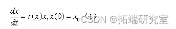
logistic The model is also called the growth retardation model , It is mainly used to describe when environmental resources are limited , The law of population growth . Due to some factors, the world population will eventually reach a saturation value . The blocking effect is reflected in the influence on , Make it decline with the increase of years . If it is expressed as a function of , Then it should be a subtractive function . Then there are
because bgistic Regression model is a generalized linear model based on binomial distribution family , So in R In software ,Logistic Regression analysis can be done by calling the generalized linear regression model function glm() To achieve , Its calling format is
Log< One glm(formula,family=binomial,data) among ,formula For the model to be fitted ,family=binomial It shows that the distribution is binomial ,data For selectable data frames .
By accessing relevant data on the world bank website , We will 1950 Year to 2100 Enter the population data of , And call glmnet Package to fit .
summary(lg.glm)
plot(x, y, main = " Population changes with years logistic curve ",xlab = " year ", ylab = " Population ( One hundred billion )")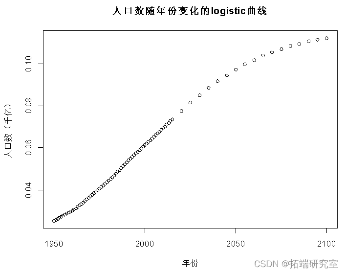
Deviance Residuals:
Min 1Q Median 3Q Max
-0.089181 -0.028946 0.002154 0.027206 0.042212
Coefficients:
Estimate Std. Error z value Pr(>|z|)
(Intercept) -23.76776 22.17527 -1.072 0.284
x 0.01046 0.01101 0.950 0.342
(Dispersion parameter for binomial family taken to be 1)
Null deviance: 0.923810 on 82 degrees of freedom
Residual deviance: 0.082928 on 81 degrees of freedom
AIC: 13.991
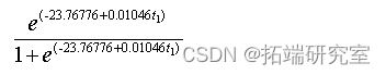
Number of Fisher Scoring iterations: 6It can be seen from the test results that the number of people can be affected over time , And the older the year , The greater the population density ; It will eventually stay at a saturation value , And get the logistic The regression model :
Model two : AFRIMA Model
Time series model can be divided into segment memory model and long memory model . The general time series analysis model has autoregression (AR) Model 、 moving average (MA) Model 、 Autoregressive moving average (ARMA) Model 、 Autoregressive integrated moving average (ARIMA) Model, etc , These models are mainly short memory models . at present , People's Empirical Research on macroeconomic variables has found , Although the long memory model has little dependence between long-distance observations, it still has research value . Fractional autoregressive moving average model (ARFMA) The model is a long memory model , It is from Granger and Joyeux (1980) as well as Hosking (1981) stay ARIMA Based on the model , It is widely used in economic and financial fields .
AFRIMA Model definition
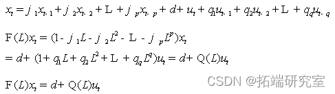
AFRIMA The model is based on A R M A Models and ARIMA Model .
ARMA(p,q), The form of the model is :
Model implementation :
 arfi(Diut[,2][)# establish arfima Model
plot(Discnt[,1],Dscunt[,2])# Raw data
points(Dicount[,1][1:66],f$fittedcol="red")# Fitting data 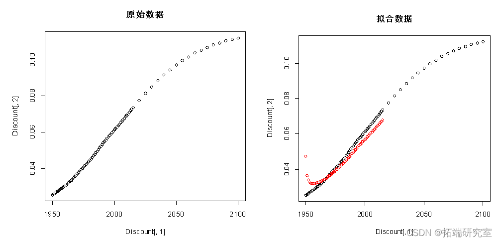

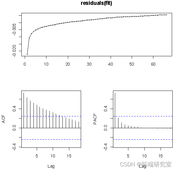
From the result of the residual diagram ,ACF The value of is not within the dotted line , Namely, the residual error is unstable , Not white noise , So let's make a first-order difference to the data .
Model stability improvement
The first-order difference of the data makes the data more stable .
points(c(2016:2100), diffinv(pre$mean)[-1]+ Discount[66,2],col="blue")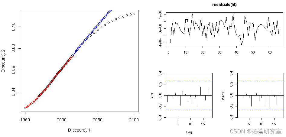
From the result of the residual diagram ,ACF The value of and PACF The values of are all within the dotted line , That is, the residual error is stable , So the model is stable .
Model three : ARIMA Model
ARIMA Model definition
ARIMA The model is called differential autoregressive moving average model . It was written by boxy and Jenkins in 70 A famous time series prediction method proposed in the early s , Bokesi - Jenkins method . among ARIMA(p,d,q) It is called differential autoregressive moving average model ,AR It's autoregression ,p Is the autoregressive term ;MA For moving average ,q Is the moving average number of items ,d It is the difference number of times when the time series becomes stationary .
ARIMA The basic idea of the model is : The data sequence formed by the prediction object over time is regarded as a random sequence , Use a certain mathematical model to approximately describe this sequence . Once the model is identified, it can predict the future value from the past value and current value of the time series .
ARIMA The basic idea of the model is : The data sequence formed by the prediction object over time is regarded as a random sequence , Use a certain mathematical model to approximately describe this sequence . Once the model is identified, it can predict the future value from the past value and current value of the time series .
The modeling process mainly includes :
First step : Autoregressive process
Make Yt Express t In the period of GDP. If we put Yt The model of is written as
(Y_t-δ)=α_1 (Y_(t-1)-δ)+u_t
among δ yes Y The average of , and ut It has zero mean and constant variance σ^2 Uncorrelated random error term of ( namely ut It's white noise ), Then Cheng Yt Follow a first-order autoregressive or AR(1) random process .
P The form of order autoregressive function is written as :
(Y_t-δ)=α_1 (Y_(t-1)-δ)+α_2 (Y_(t-2)-δ)+α_3 (Y_(t-3)-δ)+⋯+α_p2 (Y_(t-p)-δ)+u_t
There are only Y This variable , There are no other variables . Can be interpreted as “ Let the data speak for themselves ”.
The second step : Moving average process
Above AR The process is not to produce Y The only possible mechanism . If Y The model of is described as
Y_t=μ+β_0 u_t+β_1 u_(t-1)
among μ Is constant ,u White noise ( Zero mean 、 Constant variance 、 Non autocorrelation ) Random error term .t In the period of Y Equal to a constant plus a moving average of the present and past error terms . said Y Follow a first-order moving average or MA(1) The process .
q The order moving average can be written as :
Y_t=μ+β_0 u_t+β_1 u_(t-1)+β_2 u_(t-2)+⋯+β_q u_(t-q)
Self regressive moving average process
If Y Both AR and MA Characteristics of , It is ARMA The process .Y It can be written.
Y_t=θ+α_1 Y_(t-1)+β_0 u_t+β_1 u_(t-1)
There is an autoregressive term and a moving average term , So he's a ARMA(1,1) The process .Θ It's a constant term .
ARMA(p,q) In the process p An autoregressive sum q Moving average .
The third step : Autoregressive quadrature moving average process
All the above is based on the fact that the data is stable , But many times the time data is non-stationary , That is, single integer ( Simple product ) Of , Generally, nonstationary data can be obtained by difference . So if we talk about a time series difference d Time , Become stable , And then use AEMA(p,q) Model , Then we say that the original time series is AEIMA(p,d,q), Autoregressive quadrature moving average time series .AEIMA(p,0,q)=AEMA(p,q).

Usually ,ARIMA The modeling steps are 4 Stages : Sequence stationarity test , Preliminary identification of the model , Model parameter estimation and model diagnosis analysis .
Model implementation
Step one : distinguish . Find the right p、d、 and q value . It can be solved by correlation diagram and partial correlation diagram .
Step two : It is estimated that . Estimate the parameters of autoregressive and moving average terms included in the model week . Sometimes the least square method can be used , Sometimes it is necessary to use nonlinear estimation methods .( The software can automatically complete )
Step three : The diagnosis ( test ). See if the calculated residual is white noise , yes , Then accept the fitting ; No , Then do it again .
Step four : forecast . More reliable in the short term .
say concretely :
First , See if there is any obvious trend, Do you need differencing Then model .
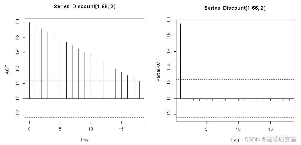
from ACF and PACF As a result , The sequence did not fall within the dotted line quickly , therefore , The sequence is unstable . The sequence is differentiated .
Draw ACF and PACF, Decide which model to use by looking at the picture (ARMA(p,q),ARIMA And so on. ).
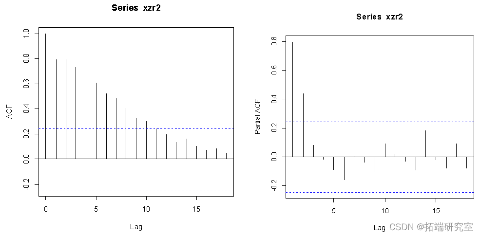
From the data results after the difference ,ACF stay 8 After the step, it begins to fall into the dotted line ,PACF stay 2 The step will soon fall into the dotted line , therefore p=8,q=2,d=1.
xz1=automa(Dist[1:66,2],ic=c('bic'),trace=T)# Automatically find the best arima Model ARIMA(2,2,2) : -1058.701
ARIMA(0,2,0) : -1026.504
ARIMA(1,2,0) : -1049.834
ARIMA(0,2,1) : -1048.83
ARIMA(1,2,2) : -1062.532
ARIMA(1,2,1) : -1050.673
ARIMA(1,2,3) : -1058.723
ARIMA(2,2,3) : Inf
ARIMA(0,2,2) : -1060.99
Best model: ARIMA(1,2,2) 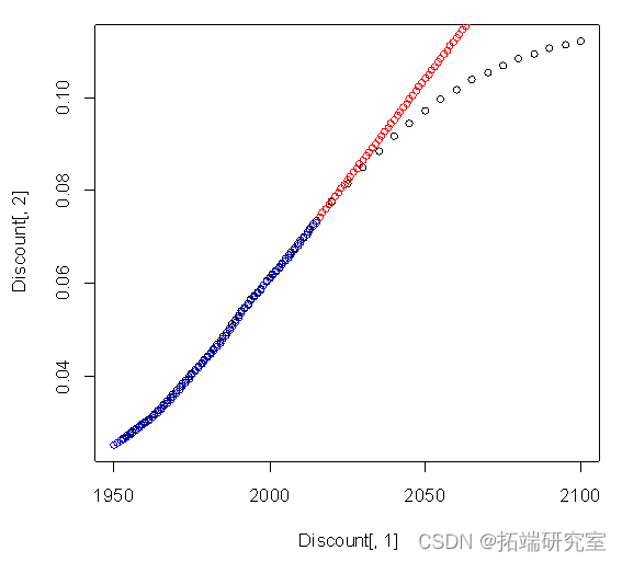
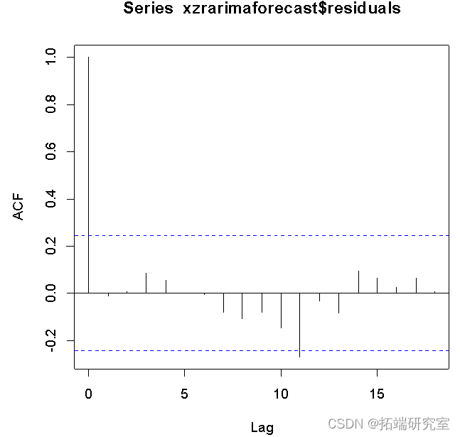
From the residual ACF As a result , The sequence quickly and stably falls into the dotted line range , The model is stable .
plot(Discnt[,1],Disnt[,2])
points(c(2016:2100) ,Diunt[66,2]+diffinv(xzrcast$mean)[-1],col="red")# Predictive value 2015 To 2100 year 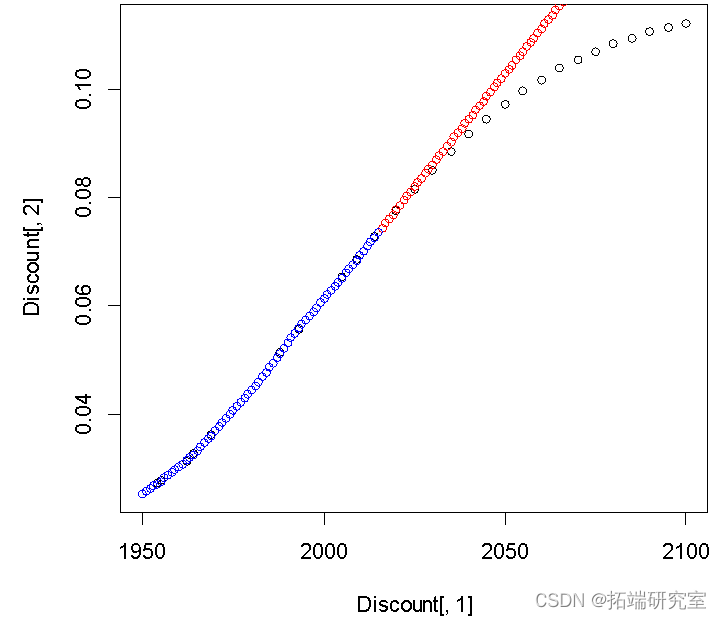
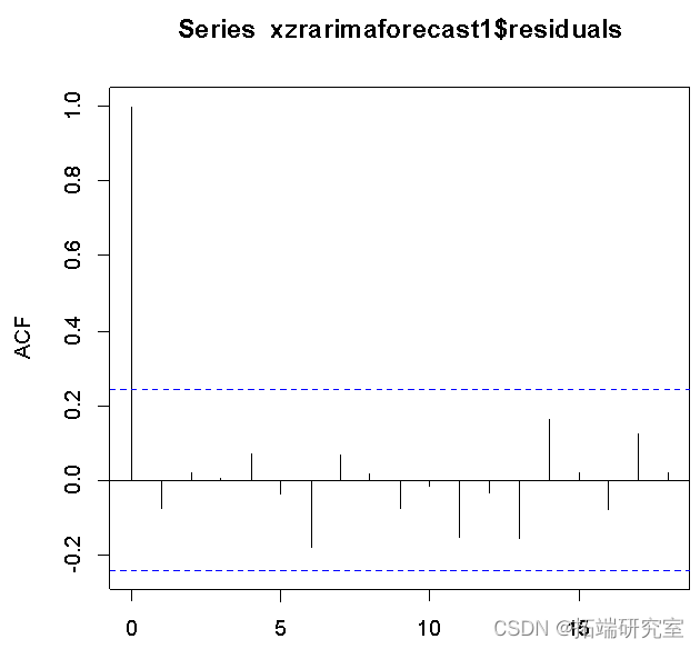
From the residual ACF As a result , The sequence quickly and stably falls into the dotted line range , The model is stable .
In order to test that the prediction error is a normal distribution with zero mean , We can draw the histogram of prediction error , And the average value is zero 、 Plot of normal distribution of standard variance to prediction error .
points(mst$mids, myst$density, type="l", col="blue", lwd=2)
}
plotForecrrors(xzrrecast $residuals)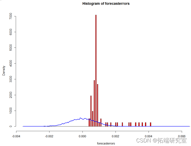
reference
【1】 Statistical simulation and its R Realization , Xiao Zhihong , Wuhan university press
【2】Logistic Application of model in population prediction , Yan Huizhen , Journal of Dalian University of Technology , The first 27 Volume No 4 period

The most popular insights
2.R Language GARCH-DCC Models and DCC(MVT) Modeling estimation
3.R Language implementation Copula Algorithm modeling dependency case analysis report
4.R Language COPULAS And financial time series data VaR analysis
5.R Language diversity COPULA GARCH Model time series prediction
6. use R Language implementation of neural network to predict the stock example
7.r The realization of language prediction volatility :ARCH Model and HAR-RV Model
8.R How language makes Markov transformation model markov switching model
边栏推荐
- The perfect car for successful people: BMW X7! Superior performance, excellent comfort and safety
- Interpretation of mask RCNN paper
- Pytorch common code snippet collection
- 微信小程序;胡言乱语生成器
- [swagger]-swagger learning
- Take you ten days to easily complete the go micro service series (IX. link tracking)
- Take you ten days to easily complete the go micro service series (IX. link tracking)
- PowerShell:在代理服务器后面使用 PowerShell
- 流批一体在京东的探索与实践
- Global and Chinese market of nutrient analyzer 2022-2028: Research Report on technology, participants, trends, market size and share
猜你喜欢

"2022" is a must know web security interview question for job hopping

Wechat applet: exclusive applet version of the whole network, independent wechat community contacts
Exploration and practice of integration of streaming and wholesale in jd.com
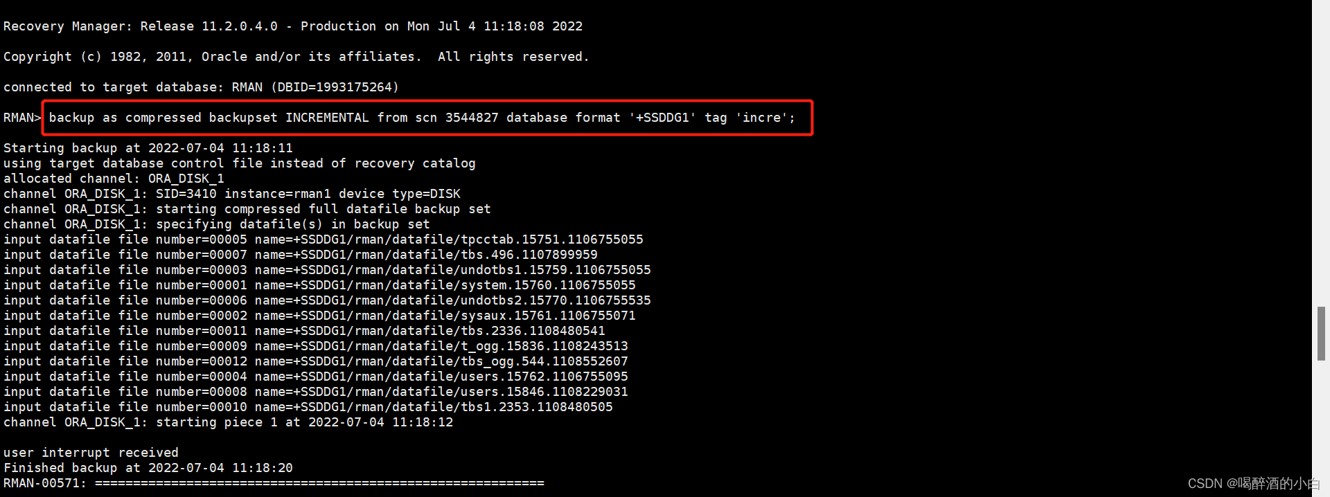
Incremental backup? db full

One plus six brushes into Kali nethunter
Take you ten days to easily complete the go micro service series (IX. link tracking)
One plus six brushes into Kali nethunter

After reading the average code written by Microsoft God, I realized that I was still too young
Redis(1)之Redis简介
![[flutter topic] 64 illustration basic textfield text input box (I) # yyds dry goods inventory #](/img/1c/deaf20d46e172af4d5e11c28c254cf.jpg)
[flutter topic] 64 illustration basic textfield text input box (I) # yyds dry goods inventory #
随机推荐
Phpstrom setting function annotation description
PHP 基础篇 - PHP 中 DES 加解密详解
Basic operation of database and table ----- phased test II
Wechat applet: independent background with distribution function, Yuelao office blind box for making friends
C basic knowledge review (Part 3 of 4)
Delaying wages to force people to leave, and the layoffs of small Internet companies are a little too much!
Mysql database | build master-slave instances of mysql-8.0 or above based on docker
Es uses collapsebuilder to de duplicate and return only a certain field
实战模拟│JWT 登录认证
batchnorm. Py this file single GPU operation error solution
Jcenter () cannot find Alibaba cloud proxy address
Wechat applet: wechat applet source code download new community system optimized version support agent member system function super high income
Four pits in reentrantlock!
Win: use PowerShell to check the strength of wireless signal
流批一体在京东的探索与实践
Global and Chinese markets for industrial X-ray testing equipment 2022-2028: Research Report on technology, participants, trends, market size and share
Take you ten days to easily complete the go micro service series (IX. link tracking)
PHP wechat official account development
Actual combat simulation │ JWT login authentication
【大型电商项目开发】性能压测-性能监控-堆内存与垃圾回收-39