当前位置:网站首页>Kaggle competition two Sigma connect: rental listing inquiries (xgboost)
Kaggle competition two Sigma connect: rental listing inquiries (xgboost)
2022-07-06 12:00:00 【Want to be a kite】
Kaggle competition , Website links :Two Sigma Connect: Rental Listing Inquiries

According to the data information on the rental website , Predict the popularity of the house .( This is a question of classification , Contains the following data , Variable with category 、 Integer variable 、 Text variable ).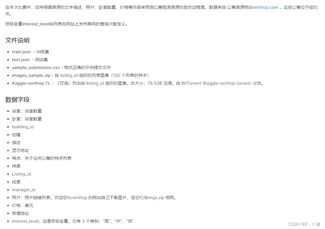
XGBoost Model
Use sklearn Complete modeling and prediction . The data set can be downloaded from the official website of the competition .
XGBoost Website
About XGBoost Explanation , I won't introduce . follow-up , A series of machine learning algorithms will be explained .
import os
import sys
import operator
import numpy as np
import pandas as pd
import zipfile
from scipy import sparse
import xgboost as xgb
from sklearn import model_selection, preprocessing, ensemble
from sklearn.metrics import log_loss
from sklearn.feature_extraction.text import TfidfVectorizer, CountVectorizer
TfidfVectorizer, CountVectorizer see sklearn Official website or TfidfVectorizer, CountVectorizer
# Data acquisition , See another article for details
train_df = pd.read_json(zipfile.ZipFile(r'E:\Kaggle\Kaggle_dataset01\two_sigma\train.json.zip').open('train.json'))
test_df = pd.read_json(zipfile.ZipFile(r'E:\Kaggle\Kaggle_dataset01\two_sigma\test.json.zip').open('test.json'))
Another article - Random forest method
# Feature Engineering
features_to_use = ['bathrooms','bedrooms','latitude','longitude','price']
train_df['num_photos'] = train_df['photos'].apply(len)
test_df['num_photos'] = test_df['photos'].apply(len)

train_df['num_features'] = train_df['features'].apply(len)
test_df['num_features'] = test_df['features'].apply(len)

train_df["num_description_words"] = train_df["description"].apply(lambda x: len(x.split(" ")))
test_df["num_description_words"] = test_df["description"].apply(lambda x: len(x.split(" ")))

train_df["created"] = pd.to_datetime(train_df["created"])
test_df["created"] = pd.to_datetime(test_df["created"])

train_df["created_year"] = train_df["created"].dt.year
test_df["created_year"] = test_df["created"].dt.year
train_df["created_month"] = train_df["created"].dt.month
test_df["created_month"] = test_df["created"].dt.month
train_df["created_day"] = train_df["created"].dt.day
test_df["created_day"] = test_df["created"].dt.day
train_df["created_hour"] = train_df["created"].dt.hour
test_df["created_hour"] = test_df["created"].dt.hour

features_to_use.extend(["num_photos", "num_features", "num_description_words","created_year", "created_month", "created_day", "listing_id", "created_hour"])

categorical = ['display_address','manager_id','building_id','street_address']
for f in categorical:
    if train_df[f].dtype == 'object':
        lbl = preprocessing.LabelEncoder()
        lbl.fit(list(train_df[f].values) + list(test_df[f].values))
        train_df[f] = lbl.transform(list(train_df[f].values))
        test_df[f] = lbl.transform(list(test_df[f].values))
        features_to_use.append(f)

train_df['features'] = train_df["features"].apply(lambda x: " ".join(["_".join(i.split(" ")) for i in x]))
test_df['features'] = test_df["features"].apply(lambda x: " ".join(["_".join(i.split(" ")) for i in x]))
print(train_df["features"].head())
tfidf = CountVectorizer(stop_words='english', max_features=200)
tr_sparse = tfidf.fit_transform(train_df["features"])
te_sparse = tfidf.transform(test_df["features"])

train_X = sparse.hstack([train_df[features_to_use], tr_sparse]).tocsr()
test_X = sparse.hstack([test_df[features_to_use], te_sparse]).tocsr()

target_num_map = {
    'high':0, 'medium':1, 'low':2}
train_y = np.array(train_df['interest_level'].apply(lambda x: target_num_map[x]))
print(train_X.shape, test_X.shape)
# Model structures,
def runXGB(train_X,train_y,test_X,test_y=None,feature_names=None,seed_val=0,num_rounds=1000):
    param = {
    }
    param['objective'] = 'multi:softprob'
    param['eta'] = 0.1
    param['max_depth'] = 6
    param['silent'] = 1
    param['num_class'] = 3
    param['eval_metric'] = "mlogloss"
    param['min_child_weight'] = 1
    param['subsample'] = 0.7
    param['colsample_bytree'] = 0.7
    param['seed'] = seed_val
    num_rounds = num_rounds

    plst = list(param.items())

    xgbtrain = xgb.DMatrix(train_X,label=train_y)

    if test_y is not None:
        xgbtest = xgb.DMatrix(test_X,label=test_y)
        watchlist = [(xgbtrain,'train'),(xgbtest,'test')]
        model =xgb.train(plst,xgbtrain,num_rounds,watchlist,early_stopping_rounds=20,evals_result=evals_result)
    else:
        xgbtest = xgb.DMatrix(test_X)
        model = xgb.train(plst,xgbtrain,num_rounds)
    pred_test_y = model.predict(xgbtest)
    return pred_test_y,model
# model training
cv_scores = []
test_loss = []
train_loss = []
evals_result = {
    }
import matplotlib.pyplot as plt
kf = model_selection.KFold(n_splits=5,shuffle=True,random_state=12)
for dev_index,val_index in kf.split(range(train_X.shape[0])):
    dev_X, val_X = train_X[dev_index,:], train_X[val_index,:]
    dev_y, val_y = train_y[dev_index], train_y[val_index]
    preds, model = runXGB(dev_X, dev_y, val_X, val_y)
    cv_scores.append(log_loss(val_y, preds))
    print(cv_scores)
    break  # Removable , take KFlold All the conditions of training once . Choose the best
# Model training prediction
preds, model = runXGB(train_X, train_y, test_X, num_rounds=400)
out_df = pd.DataFrame(preds)
out_df.columns = ["high", "medium", "low"]
out_df["listing_id"] = test_df.listing_id.values
out_df.to_csv("xgb.csv", index=False)
# Analysis of model training process (loss Trends )
import matplotlib.pyplot as plt
plt.figure(figsize=(8,4))
plt.plot(list(range(int(len(evals_result['train']['mlogloss'])))),evals_result['train']['mlogloss'],'r-',label='train_loss')
plt.plot(list(range(int(len(evals_result['test']['mlogloss'])))),evals_result['test']['mlogloss'],'b-',label='test_loss')
plt.legend(loc='upper right')
plt.show()
# Here's the picture
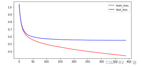
Run the above code ,XGBoost The effect of is much better than random forest , But it can continue to improve . Further improve the feature engineering part , Get better features ( Or better )!
边栏推荐
- Inline detailed explanation [C language]
- Pytoch temperature prediction
- [Kerberos] deeply understand the Kerberos ticket life cycle
- Pytoch implements simple linear regression demo
- There are three iPhone se 2022 models in the Eurasian Economic Commission database
- Reno7 60W超级闪充充电架构
- Detailed explanation of nodejs
- A possible cause and solution of "stuck" main thread of RT thread
- 第4阶段 Mysql数据库
- 优先级反转与死锁
猜你喜欢
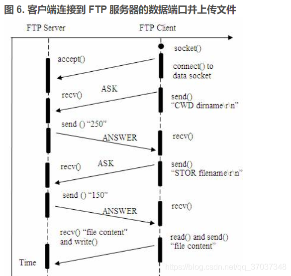
FTP file upload file implementation, regularly scan folders to upload files in the specified format to the server, C language to realize FTP file upload details and code case implementation
![[CDH] cdh5.16 configuring the setting of yarn task centralized allocation does not take effect](/img/e7/a0d4fc58429a0fd8c447891c848024.png)
[CDH] cdh5.16 configuring the setting of yarn task centralized allocation does not take effect
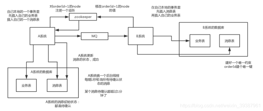
Implementation scheme of distributed transaction
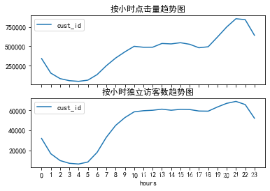
E-commerce data analysis -- User Behavior Analysis
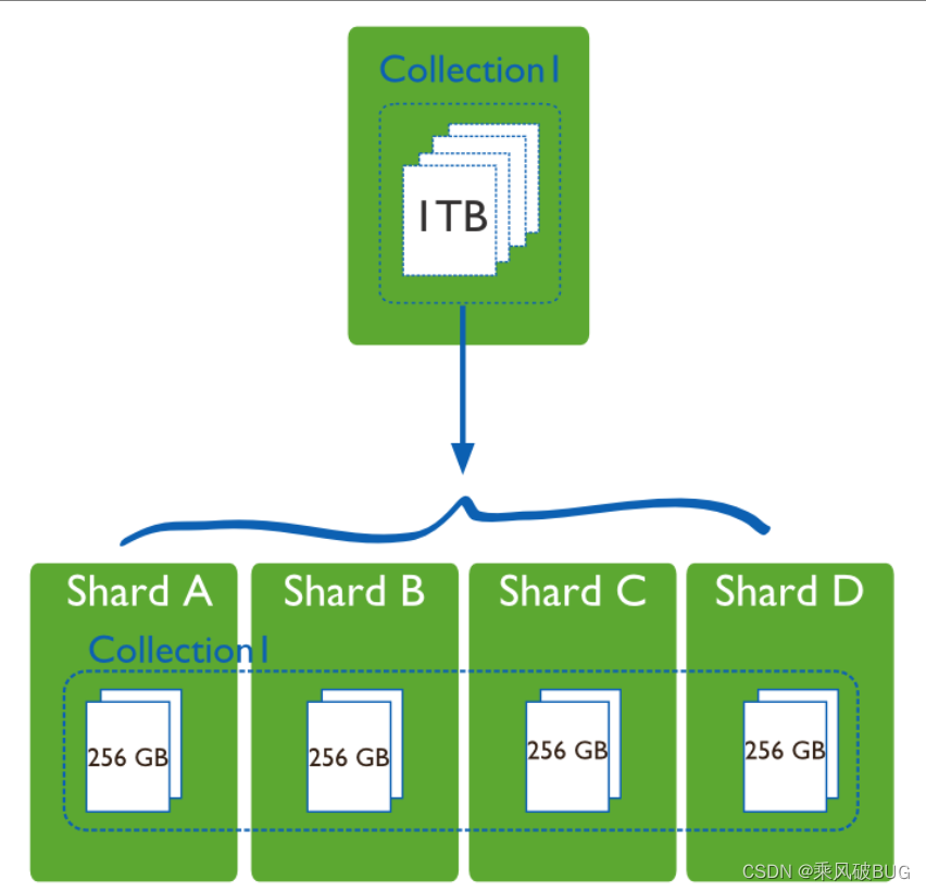
MongoDB
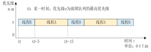
RT-Thread 线程的时间片轮询调度
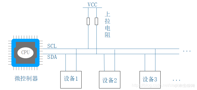
I2C总线时序详解
电商数据分析--薪资预测(线性回归)

Composition des mots (sous - total)
电商数据分析--用户行为分析
随机推荐
Unit test - unittest framework
分布式節點免密登錄
Cannot change version of project facet Dynamic Web Module to 2.3.
Missing value filling in data analysis (focus on multiple interpolation method, miseforest)
Detailed explanation of 5g working principle (explanation & illustration)
Redis面试题
Word typesetting (subtotal)
4. Install and deploy spark (spark on Yan mode)
STM32 how to locate the code segment that causes hard fault
电商数据分析--用户行为分析
Machine learning -- linear regression (sklearn)
PyTorch四种常用优化器测试
列表的使用
ESP8266通过arduino IED连接巴法云(TCP创客云)
Détails du Protocole Internet
Linux yum安装MySQL
[template] KMP string matching
4、安装部署Spark(Spark on Yarn模式)
Linux Yum install MySQL
[Kerberos] deeply understand the Kerberos ticket life cycle