Machine learning -- linear regression (sklearn)

machine learning – linear regression model （sklearn）

linear regression model Yes ： In general form Univariate linear regression and Multiple linear regression , Use L2 Norm Ridge return （Ridge）, Use L1 Norm Lasso return (Lasso), Use L1 and L2 Norm ElasticNet Return to （ It's right Lasso Fusion of regression and ridge regression ）, Logical regression .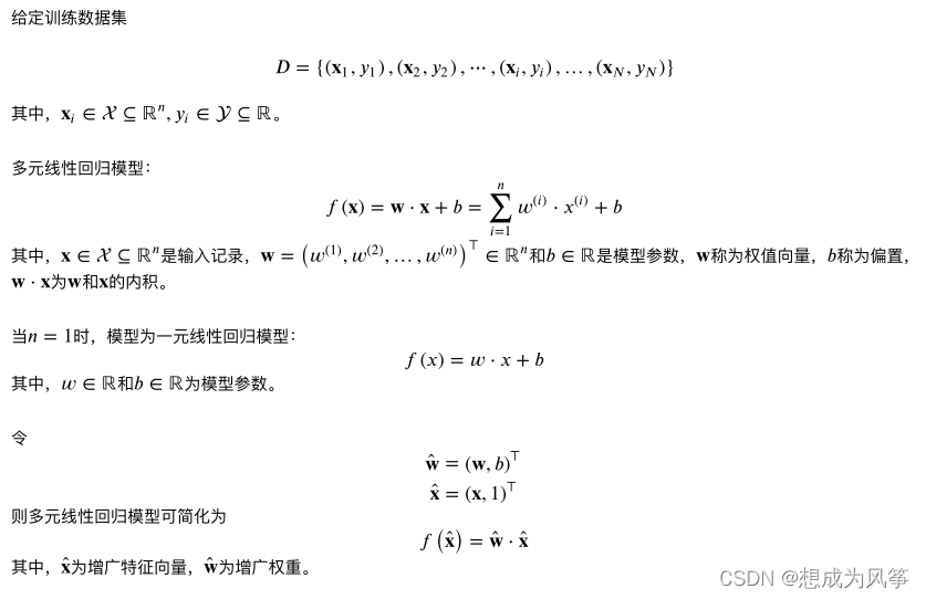

Linear regression -sklearn Library call mode and parameter interpretation ：

from sklearn.linear_model import LinearRegression
LinearRegression(fit_intercept=True,normalize=False,copy_X=True,n_jobs=1)

Parameter meaning ：

1. fit_intercept: Boolean value , Specify whether to calculate the intercept in linear regression , namely b value . If False, Then don't count b value .
2. normalize: Boolean value . If False, Then the training samples will be normalized .
3. copy_X： Boolean value . If True, Will copy a copy of training data .
4. n_jobs: An integer . Specified when tasks are parallel CPU Number . If the value is -1 Then use all available CPU.

attribute

1. coef_: The weight vector
2. intercept_: intercept b value

Method ：

1. fit(X,y)： Training models .
2. predict(X)： Use the trained model to predict , And return the predicted value .
3. score(X,y)： Return the score of prediction performance .
   The formula is ：$score=(1-u/v)$
   among $u=((y_{t}rue-y_{p}red)\ast \ast 2).sum(),v=((y_{t}rue-y_{t}rue.mean())\ast \ast 2).sum()$
   score The maximum is 1, But it may be negative ( The prediction effect is too poor ).score The bigger it is , The better the prediction performance .

Join in L2 Regularized linear regression -sklearn Library call mode and parameter interpretation

from sklearn.linear_model import Ridge
Ridge(alpha=1.0, fit_intercept=True, normalize=False,copy_X=True, max_iter=None,
tol=1e-3, solver=“auto”,random_state=None)

Parameter meaning ：

1. alpha: Coefficient of regular term , The larger the value, the larger the proportion of regular terms . The initial value is suggested to be set to 0, In this way, first determine a better study rate , Once the learning rate is determined , to alpha A smaller value , Then according to the accuracy on the verification set , Increase or decrease 10 times .10 Double coarse adjustment , When the appropriate order of magnitude is determined , Then fine adjust in the same order of magnitude .

2. fit_intercept： Boolean value , Specify whether intercept calculation is required b value .False It doesn't count b value .

3. normalize: Boolean value . If it is equal to True, The data will be normalized before model training . There are two benefits ： (1): Improve the convergence rate of the model , Reduce the time to find the optimal solution . (2) Improve the accuracy of the model .

4. copy_X: Boolean value . If set to True, Will copy a copy of training data .

5. max_iter： Integers . The maximum number of iterations is specified . If None, The default value .

6. tol: threshold . Judge whether the iteration converges or meets the accuracy requirements .

7. solver: character string . Specify the algorithm to solve the optimization problem .
   (1).solver=‘auto’, Automatic selection algorithm based on data set .
   (2).solver=‘svd’, Using the method of singular value decomposition to calculate
   (3).solver=‘cholesky’, use scipy.linalg.solve Function to solve the optimal solution .
   (4).solver=‘sparse_cg’, use scipy.sparse.linalg.cg Function to find the optimal solution .
   (5).solver=‘sag’, use Stochastic Average Gradient descent The algorithm solves the optimization problem .

8. random_state: An integer or a RandomState example , Or for None. It's in solver="sag" When using .
   (1). If it's an integer , It specifies the seed of the random number generator .
   (2). If RandomState example , The random number generator is specified .
   (3). If None, Then use the default random number generator .

attribute ：

1. coef_： The weight vector .
2. intercept_： intercept b Value .
3. n_iter_: The actual number of iterations .

Method ：

1. fit(X,y)： Training models .
2. predict(X): Use the trained model to predict , And return the predicted value .
3. score(X,y): Return the score of prediction performance .
   The formula is ：$score=(1-u/v)$
   among $u=((y_{t}rue-y_{p}red)\ast \ast 2).sum(),v=((y_{t}rue-y_{t}rue.mean())\ast \ast 2).sum()$
   score The maximum is 1, But it may be negative ( The prediction effect is too poor ).score The bigger it is , The better the prediction performance .

Join in L1 Regularized linear regression -sklearn Library call mode and parameter interpretation

from sklearn.linear_model import Lasso
Lasso(alpha=1.0, fit_intercept=True, normalize=False, precompute=False,
copy_X=True, max_iter=1000,
tol=1e-4, warm_start=False, positive=False,random_state=None,
selection=‘cyclic’)

Parameter meaning ：

1. alpha： Coefficient of regularization term
2. fit_intercept： Boolean value , Specify whether intercept calculation is required b value .False It doesn't count b value .
3. max_iter: Specify the maximum number of iterations .
4. normalize： Boolean value . If it is equal to True, The data will be normalized before model training . There are two benefits ： (1): Improve the convergence rate of the model , Reduce the time to find the optimal solution . (2) Improve the accuracy of the model .
5. precompute: A Boolean value or a sequence . It decides whether to calculate in advance Gram Matrix to speed up computation .
6. tol: threshold . Judge whether the iteration converges or meets the accuracy requirements .
7. warm_start： Boolean value . If True, Then use the results of the previous training to continue training . Or start training from scratch .
8. positive： Boolean value . If True, Then force the components of the weight vector to be positive .
9. selection: character string , It can be "cyclic" or "random". It specifies when each iteration , Choose which of the weight vectors Component to update .
   (1)“random”: When it's updated , Randomly select a component of the weight vector to update .
   (2)“cyclic”: When it's updated , Select a component of the weight vector from front to back to update
10. random_state： An integer or a RandomState example , perhaps None.
    (1): If it's an integer , It specifies the seed of the random number generator .
    (2): If RandomState example , Then it specifies the random number generator .
    (3): If None, Then use the default random number generator .

attribute ：

1. coef_： The weight vector .
2. intercept_： intercept b value .
3. n_iter_： The actual number of iterations .

Method ：

1. fit(X,y)： Training models .
2. predict(X): Using models to make predictions , Return forecast .
3. score(X,y): Return the score of prediction performance .
   The formula is ：$score=(1-u/v)$
   among $u=((y_{t}rue-y_{p}red)\ast \ast 2).sum(),v=((y_{t}rue-y_{t}rue.mean())\ast \ast 2).sum()$
   score The maximum is 1, But it may be negative ( The prediction effect is too poor ).score The bigger it is , The better the prediction performance .

ElasticNet Regression is right Lasso Fusion of regression and ridge regression , The regularization term is L1 Norm sum L2 A trade-off of norms .-sklearn Library call mode and parameter interpretation

The regularization term is : $alpha\ast l{1}_{r}atio\ast ||w|{|}_1+0.5\ast alpha\ast (1-l{1}_{r}atio)\ast ||w|{|}_2^2$

from sklearn.linear_model import ElasticNet
ElasticNet(alpha=1.0, l1_ratio=0.5, fit_intercept=True,
normalize=False,precompute=False, max_iter=1000,copy_X=True, tol=1e-4,
warm_start=False, positive=False,random_state=None, selection=‘cyclic’)

Parameter meaning ：

1. alpha: Regularization term alpha value .
2. l1_ratio: In the regularization term l1_ratio value .
3. fit_intercept: Boolean value , Specify whether intercept calculation is required b value .False It doesn't count b value .
4. max_iter： Specify the maximum number of iterations .
5. normalize： Boolean value . If it is equal to True, The data will be normalized before model training . There are two benefits ：
   (1): Improve the convergence rate of the model , Reduce the time to find the optimal solution .
   (2) Improve the accuracy of the model .
6. copy_X: Boolean value . If set to True, Will copy a copy of training data .
7. precompute: A Boolean value or a sequence . It decides whether to calculate in advance Gram Matrix to speed up computation .
8. tol: threshold . Judge whether the iteration converges or meets the accuracy requirements .
9. warm_start: Boolean value . If True, Then use the results of the previous training to continue training . Or start training from scratch .
10. positive: Boolean value . If True, Then force the components of the weight vector to be positive .
11. selection: character string , It can be "cyclic" or "random". It specifies when each iteration , Choose which of the weight vectors Components to update .
    (1)“random”: When it's updated , Randomly select a component of the weight vector to update .
    (2)“cyclic”: When it's updated , Select a component of the weight vector from front to back to update .
12. random_state: An integer or a RandomState example , perhaps None.
    (1): If it's an integer , It specifies the seed of the random number generator .
    (2): If RandomState example , Then it specifies the random number generator .
    (3): If None, Then use the default random number generator .

attribute ：

1. coef_： The weight vector .
2. intercept_： intercept b value .
3. 3.n_iter_： The actual number of iterations .

Method ：

1. fit(X,y)： Training models .
2. predict(X): Using models to make predictions , Return forecast .
3. score(X,y): Return the score of prediction performance .

The formula is ：$score=(1-u/v)$
among $u=((y_{t}rue-y_{p}red)\ast \ast 2).sum(),v=((y_{t}rue-y_{t}rue.mean())\ast \ast 2).sum()$
score The maximum is 1, But it may be negative ( The prediction effect is too poor ).score The bigger it is , The better the prediction performance .

Logical regression -sklearn Library call mode and parameter interpretation

from sklearn.linear_model import LogisticRegression
LogisticRegression(penalty=‘l2’,dual=False,tol=1e-4,C=1.0,
fit_intercept=True,intercept_scaling=1,class_weight=None,
random_state=None,solver=‘liblinear’,max_iter=100,
multi_class=‘ovr’,verbose=0,warm_start=False,n_jobs=1)

Parameter meaning ：

1. penalty: character string , The regularization strategy is specified . The default is "l2"
   (1) If "l2", Then the objective function of optimization is ：$0.5\ast ||w|{|}_2^2+C\ast L(w),C>0$, L(w) Is the maximum likelihood function .
   (2) If "l1", Then the objective function of optimization is $||w|{|}_1+C\ast L(w),C>0$, L(w) Is the maximum likelihood function .
2. dual: Boolean value . The default is False. If it is equal to True, Then solve its dual form .
   Only in penalty="l2" also solver="liblinear" Only when there is a dual form . If False, Then solve the original form . When n_samples > n_features, In favor of dual=False.
3. tol: threshold . Judge whether the iteration converges or meets the accuracy requirements .
4. C:float, The default is 1.0. Specifies the reciprocal of the coefficient of the regularization term . Must be a positive floating point number .C The smaller the value. , The larger the regularization term .
5. fit_intercept:bool value . The default is True. If False, You won't calculate b value .
6. intercept_scaling：float, default 1. Only when solver="liblinear" also fit_intercept=True when , It makes sense . under these circumstances , It is equivalent to adding a feature in the last column of training data , The characteristic is constant 1. Its corresponding weight is b.
7. class_weight：dict or ‘balanced’, default: None.
   (1) If it's a dictionary , Then give the weight of each classification . according to {class_label: weight} This form .
   (2) If it is "balanced"： Then the weight of each classification is inversely proportional to the frequency of the classification in the sample set .
   $n_{s}amples/(n_{c}lasses\ast np.bincount(y))$
   (3) If not specified , Then the weight of each classification is 1.
8. random_state: int, RandomState instance or None, default: None
   (1): If it's an integer , It specifies the seed of the random number generator .
   (2): If RandomState example , Then it specifies the random number generator .
   (3): If None, Then use the default random number generator .
9. solver: character string , Specify the algorithm to solve the optimization problem .
   {‘newton-cg’, ‘lbfgs’, ‘liblinear’, ‘sag’, ‘saga’},default: ‘liblinear’
   (1)solver=‘liblinear’, For small data sets ,'liblinear’ It's a good choice . For large data sets ,‘sag’ and ’saga’ Faster processing .
   (2)solver=‘newton-cg’, Adopt Newton method
   (3)solver=‘lbfgs’, use L-BFGS Quasi Newton method .
   (4)solver=‘sag’, use Stochastic Average Gradient descent Algorithm .
   (5) For multi classification problems , Only ’newton-cg’,‘sag’,'saga’ and ’lbfgs’ Dealing with multiple losses ;
   ‘liblinear’ Is limited to ’ovr’ programme .
   (6)newton-cg’, ‘lbfgs’ and ‘sag’ Can only handle L2 penalty,‘liblinear’ and ‘saga’ Can deal with L1 penalty.
10. max_iter: Specify the maximum number of iterations .default: 100. Only right ’newton-cg’, ‘sag’ and 'lbfgs’ apply .
11. multi_class：{‘ovr’, ‘multinomial’}, default: ‘ovr’. Specify the strategy for classification problems .
    (1)multi_class=‘ovr’, use ’one_vs_rest’ Strategy .
    (2)multi_class=‘multinomal’, Adopt multiple classification logistic regression strategy directly .
12. verbose: It is used to turn on or off the iteration intermediate output log function .
13. warm_start: Boolean value . If True, Then use the results of the previous training to continue training . Or start training from scratch .
14. n_jobs: int, default: 1. When specifying tasks in parallel CPU Number . If -1, Then use all available CPU.

attribute ：

1. coef_： The weight vector .
2. intercept_： intercept b value .
3. n_iter_： The actual number of iterations .

Method ：

1. fit(X,y): Training models .
2. predict(X): Use the trained model to predict , And return the predicted value .
3. predict_log_proba(X): Returns an array , The array elements, in turn, are X The logarithm of the probability predicted for each category .
4. predict_proba(X): Returns an array , The array elements, in turn, are X Prediction is the probability value of each category .
5. score(X,y): Returns the accuracy of the forecast .

Practical cases ：

Multiple linear regression

import matplotlib.pyplot as plt
import numpy as np
import pandas as pd
from sklearn import datasets,linear_model,model_selection
from sklearn.model_selection import train_test_split
def load_data():
    diabetes = datasets.load_diabetes()
    return train_test_split(diabetes.data,diabetes.target,test_size=0.2)

def test_LineearRegression(*data):
    X_train,X_test,y_train,y_test = data
    regr = linear_model.LinearRegression()
    regr.fit(X_train,y_train)
    print('Coefficients:{},intercept:{}'.format(regr.coef_,regr.intercept_))
    print('Residual sum of squares:{}'.format(np.mean(regr.predict(X_test)-y_test)**2))
    print('Scores:{}'.format(regr.score(X_test,y_test)))
    
if __name__ == '__main__':
    X_train,X_test,y_train,y_test = load_data()
    test_LineearRegression(X_train,X_test,y_train,y_test)

Lasso Return to

import matplotlib.pyplot as plt
import numpy as np
from sklearn import datasets,linear_model
from sklearn.model_selection import train_test_split

def load_data():
    diabetes = datasets.load_diabetes()
    return train_test_split(diabetes.data,diabetes.target,test_size=0.2)

def test_Lasso(*data):
    X_train,X_test,y_train,y_test = data
    regr = linear_model.Lasso()
    regr.fit(X_train,y_train)
    print('Coefficients:{},intercept:{}'.format(regr.coef_,regr.intercept_))
    print('Residual sum of squares:{}'.format(np.mean(regr.predict(X_test)-y_test)**2))
    print('Scores:{}'.format(regr.score(X_test,y_test)))
    
def test_Lasso_alpha(*data):
    X_train,X_test,y_train,y_test = data
    alphas = [0.01,0.02,0.05,0.1,0.2,0.5,1,2,5,10,20,50,100,200,500,1000]
    scores = []
    for i,alpha in enumerate(alphas):
        regr = linear_model.Lasso(alpha=alpha)
        regr.fit(X_train,y_train)
        scores.append(regr.score(X_test,y_test))
    
    fig = plt.figure()
    ax = fig.add_subplot(1,1,1)
    ax.plot(alphas,scores)
    ax.set_xlabel("alpha")
    ax.set_ylabel("score")
    ax.set_xscale("log")
    ax.set_title('Lasso')
    plt.show()
    
if __name__ == '__main__':
    X_train,X_test,y_train,y_test = load_data()
    test_Lasso(X_train,X_test,y_train,y_test)
    test_Lasso_alpha(X_train,X_test,y_train,y_test)
    

Ridge return （Ridge）

import matplotlib.pyplot as plt
import numpy as np
from sklearn import datasets,linear_model
from sklearn.model_selection import train_test_split

def load_data():
    diabetes = datasets.load_diabetes()
    return train_test_split(diabetes.data,diabetes.target,test_size=0.2,random_state=0)

def test_Ridge(*data):
    X_train,X_test,y_train,y_test = data
    regr = linear_model.Ridge()
    regr.fit(X_train,y_train)
    print('Coefficients:{},intercept:{}'.format(regr.coef_,regr.intercept_))
    print('Residual sum of squares:{}'.format(np.mean(regr.predict(X_test)-y_test)**2))
    print('Scores:{}'.format(regr.score(X_test,y_test)))
    
def test_Ridge_alpha(*data):
    X_train,X_test,y_train,y_test = data
    alphas = [0.01,0.02,0.05,0.1,0.2,0.5,1,2,5,10,20,50,100,200,500,1000]
    scores = []
    for i,alpha in enumerate(alphas):
        regr = linear_model.Lasso(alpha=alpha)
        regr.fit(X_train,y_train)
        scores.append(regr.score(X_test,y_test))
    
    fig = plt.figure()
    ax = fig.add_subplot(1,1,1)
    ax.plot(alphas,scores)
    ax.set_xlabel("alpha")
    ax.set_ylabel("score")
    ax.set_xscale("log")
    ax.set_title('Ridge')
    plt.show()
    
if __name__ == '__main__':
    X_train,X_test,y_train,y_test = load_data()
    test_Ridge(X_train,X_test,y_train,y_test)
    test_Ridge_alpha(X_train,X_test,y_train,y_test)

Logical regression

from math import exp
import numpy as np
import pandas as pd
import matplotlib.pyplot as plt
%matplotlib inline
from sklearn.datasets import load_iris
from sklearn.model_selection import train_test_split

def create_data():
    iris = load_iris()
    df = pd.DataFrame(iris.data,columns=iris.feature_names)
    df['label'] = iris.target
    df.columns =['sepal length', 'sepal width', 'petal length', 'petal width', 'label']
    data = np.array(df.iloc[:100,[0,1,-1]])
    return data[:,:2],data[:,-1]

X,y = create_data()
X_train,X_test,y_train,y_test = train_test_split(X,y,test_size=0.3)

class LogisticRegressionClassifier(): # Custom method 
    def __init__(self,max_iter=700,learning_rate=0.01):
        self.max_iter = max_iter
        self.learning_rate = learning_rate
    
    def sigmoid(self,x):
        return x / (1+exp(-1))
    
    def data_matrix(self,X):
        data_mat = []
        for d in X:
            data_mat.append([1.0,*d])
        return data_mat
    
    def fit(self, X, y):
        data_mat = self.data_matrix(X)
        self.weights = np.zeros((len(data_mat[0]), 1), dtype=np.float32)
        
        for iter_ in range(self.max_iter):
            for i in range(len(X)):
                result = self.sigmoid(np.dot(data_mat[i], self.weights))
                error = y[i] - result
                self.weights += self.learning_rate * error * np.transpose([data_mat[i]])
        print('LogisticRegression Model(learning_rate={}, max_iter={})'.
                            format(self.learning_rate, self.max_iter))

    def score(self, X_test, y_test):
        right = 0
        X_test = self.data_matrix(X_test)
        for x, y in zip(X_test, y_test):
            result = np.dot(x, self.weights)
            if (result > 0 and y == 1) or (result < 0 and y == 0):
                right += 1
        return right / len(X_test)
 
lr_clf = LogisticRegressionClassifier()
lr_clf.fit(X_train, y_train)
lr_clf.score(X_test, y_test)
x_points = np.arange(4, 8)
y_ = -(lr_clf.weights[1] * x_points + lr_clf.weights[0]) / lr_clf.weights[2]
plt.plot(x_points, y_)
plt.scatter(X[:50, 0], X[:50, 1], label='0')
plt.scatter(X[50:, 0], X[50:, 1], label='1')
plt.legend()     

# Call mode 
Logitic_model = linear_model.LogisticRegression()
Logitic_model.fit(X_train,y_train)     

Logitic_model.score(X_test,y_test)