PyTorch nn.RNN 参数全解析

一、简介

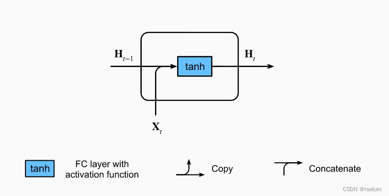
torch.nn.RNN 用于构建循环层，其中的计算规则如下：

$${\mathbf{h}}_t=\tanh ({\mathbf{W}}_{ih}{\mathbf{x}}_t+{\mathbf{b}}_{ih}+{\mathbf{W}}_{hh}{\mathbf{h}}_{t-1}+{\mathbf{b}}_{hh})\text{\hspace{1em}(1)}$$

其中 ${\mathbf{h}}_t$ 是 $t$ 时刻的隐层状态，${\mathbf{x}}_t$ 是 $t$ 时刻的输入。下标 $i$ 是 $input$ 的简写，下标 $h$ 是 $hidden$ 的简写。$\mathbf{W},\mathbf{b}$ 分别是权重和偏置。

二、前置知识

先回顾一下普通的神经网络，我们在训练它的过程中通常会投喂一小批量的数据。不妨设 $\text{batch\_size}=N$，则投喂的数据的形式为：

$$\mathbf{X}={\left[\begin{array}{c}{\mathbf{x}}_1^{\text{T}}\\ ⋮\\ {\mathbf{x}}_N^{\text{T}}\end{array}\right]}_{N\times d}$$

其中 ${\mathbf{x}}_i=(x_{i1},x_{i2},\cdots ,x_{id}{)}^{\text{T}}$ 为特征向量，维数为 $d$。

在处理序列问题中，我们会将词元转化成对应的特征向量。例如在处理一个英文句子时，我们通常会通过某种手段将每个单词转化为合适的特征向量。设序列（句子）长度为 $L$，于是在此情景下，一个句子可以表示为：

$${\text{seq}}_i={\left[\begin{array}{c}{\mathbf{x}}_{i1}^{\text{T}}\\ ⋮\\ {\mathbf{x}}_{iL}^{\text{T}}\end{array}\right]}_{L\times d}$$

其中的每个 ${\mathbf{x}}_{ij},j=1,\cdots ,L$ 都对应了句子 ${\text{seq}}_i$ 中的一个单词。在上述约定下，我们在 $t$ 时刻投喂给RNN的数据为：

$${\mathbf{X}}_t={\left[\begin{array}{c}{\mathbf{x}}_{1t}^{\text{T}}\\ ⋮\\ {\mathbf{x}}_{Nt}^{\text{T}}\end{array}\right]}_{N\times d}\text{\hspace{1em}(2)}$$

从而 $(1)$ 式改写为

$${\mathbf{H}}_t=\tanh ({\mathbf{X}}_t{\mathbf{W}}_{ih}+{\mathbf{b}}_{ih}+{\mathbf{H}}_{t-1}{\mathbf{W}}_{hh}+{\mathbf{b}}_{hh})\text{\hspace{1em}(3)}$$

其中 ${\mathbf{H}}_t,{\mathbf{H}}_{t-1}$ 的形状为 $N\times h$，${\mathbf{W}}_{ih}$ 的形状为 $d\times h$，${\mathbf{W}}_{hh}$ 的形状为 $h\times h$，${\mathbf{b}}_{ih},{\mathbf{b}}_{hh}$ 的形状为 $1\times h$，求和时利用广播机制。

在 nn.RNN 中，我们是一次性将所有时刻的数据全部投喂进去，数据形式为：

$$\mathbf{X}=[{\text{seq}}_1,{\text{seq}}_2,\cdots ,{\text{seq}}_N{]}_{N\times L\times d}\text{or}\mathbf{X}=[{\mathbf{X}}_1,{\mathbf{X}}_2,\cdots ,{\mathbf{X}}_L{]}_{L\times N\times d}$$

其中左边代表 batch_first=True 的情形，右边代表 batch_first=False 的情形。

注意： 在一个 batch 中，所有 sequence 的长度要保持相同，即 $L$ 需一致。

三、解析

3.1 所有参数

有了前置知识后，我们就能很方便的解释这些参数了。

• input_size：即 $d$；
• hidden_size：即 $h$；
• num_layers：即RNN的层数。默认是 $1$ 层。该参数大于 $1$ 时，会形成 Stacked RNN，又称多层RNN或深度RNN；
• nonlinearity：即非线性激活函数。可以选择 tanh 或 relu，默认是 tanh；
• bias：即偏置。默认启用，可以选择关闭；
• batch_first：即是否选择让 batch_size 作为输入的形状中的第一个参数。当 batch_first=True 时，输入应具有 $N\times L\times d$ 这样的形状，否则应具有 $L\times N\times d$ 这样的形状。默认是 False；
• dropout：即是否启用 dropout。如要启用，则应设置 dropout 的概率，此时除最后一层外，RNN的每一层后面都会加上一个dropout层。默认是 $0$，即不启用；
• bidirectional：即是否启用双向RNN，默认关闭。

3.2 输入参数

这里我们只考虑有 batch 的情况。

当 batch_first=True 时，输入 input 应具有形状 $N\times L\times d$，否则应具有形状 $L\times N\times d$。

h_0 为初始时刻的隐状态。当RNN为单向RNN时，h_0 的形状应为 $\text{num\_layers}\times N\times h$；当RNN为双向RNN时，h_0 的形状应为 $(2\cdot \text{num\_layers})\times N\times h$。如不提供该参数的值，则默认为全0张量。

3.3 输出参数

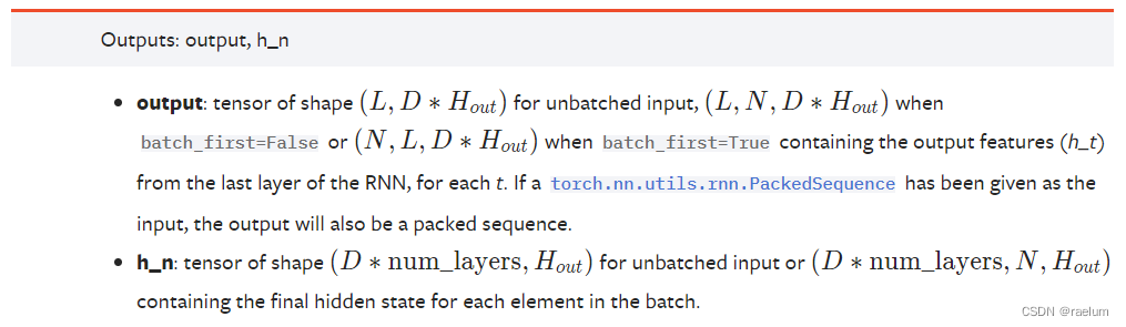
这里我们只考虑有 batch 的情况。

当RNN为单向RNN时：若 batch_first=True，输出 output 具有形状 $N\times L\times h$，否则具有形状 $L\times N\times h$。当 batch_first=False 时，output[t, :, :] 代表时刻 $t$ 时，RNN最后一层（之所以用最后一层这个术语是因为有可能出现Stacked RNN情形）的输出 ${\mathbf{h}}_t$。h_n 代表最终的隐状态，形状为 $\text{num\_layers}\times N\times h$。

当RNN为双向RNN时：若 batch_first=True，输出 output 具有形状 $N\times L\times 2h$，否则具有形状 $L\times N\times 2h$。h_n 的形状为 $(2\cdot \text{num\_layers})\times N\times h$。

事实上，对于单向RNN，有

$$\text{output}=[{\mathbf{H}}_1,{\mathbf{H}}_2,\cdots ,{\mathbf{H}}_L{]}_{L\times N\times h},\text{h\_n}=[{\mathbf{H}}_L{]}_{1\times N\times h}$$

四、通过例子来进一步理解 nn.RNN

以单隐层单向RNN为例（接下来的例子都默认 batch_first=False）。

假设有一个英文句子：He ate an apple.，忽略 . 并设置词元为单词（word）时，该序列的长度为 $4$。简便起见，我们假设每个词元都对应了一个 $6$ 维的特征向量，则上述的序列可写成：

import torch
import torch.nn as nn

torch.manual_seed(42)
seq = torch.randn(4, 6)  # 只是为了举例
print(seq)
# tensor([[ 1.9269, 1.4873, 0.9007, -2.1055, 0.6784, -1.2345],
# [-0.0431, -1.6047, 0.3559, -0.6866, -0.4934, 0.2415],
# [-1.1109, 0.0915, -2.3169, -0.2168, -0.3097, -0.3957],
# [ 0.8034, -0.6216, -0.5920, -0.0631, -0.8286, 0.3309]])

将这个句子视为一个 batch，即（注意形状为 $L\times N\times d$）：

inputs = seq.unsqueeze(1)
print(inputs)
# tensor([[[ 1.9269, 1.4873, 0.9007, -2.1055, 0.6784, -1.2345]],
# [[-0.0431, -1.6047, 0.3559, -0.6866, -0.4934, 0.2415]],
# [[-1.1109, 0.0915, -2.3169, -0.2168, -0.3097, -0.3957]],
# [[ 0.8034, -0.6216, -0.5920, -0.0631, -0.8286, 0.3309]]])
print(inputs.shape)
# torch.Size([4, 1, 6])

有了 inputs，我们还需要初始化隐状态 h_0，不妨设 $h=3$：

h_0 = torch.randn(1, 1, 3)
print(h_0)
# tensor([[[ 1.3525, 0.6863, -0.3278]]])

接下来创建RNN层，事实上只需要输入 input_size 和 hidden_size 即可：

rnn = nn.RNN(6, 3)

观察输出：

outputs, h_n = rnn(inputs, h_0)
print(outputs)
# tensor([[[-0.5428, 0.9207, 0.7060]],
# [[-0.2245, 0.2461, -0.4578]],
# [[ 0.5950, -0.3390, -0.4598]],
# [[ 0.9281, -0.7660, 0.5954]]], grad_fn=<StackBackward0>)
print(h_n)
# tensor([[[ 0.9281, -0.7660, 0.5954]]], grad_fn=<StackBackward0>)

五、从零开始手写一个单隐层单向RNN

首先写好框架：

class RNN(nn.Module):

    def __init__(self, input_size, hidden_size):
        super().__init__()
        pass

    def forward(self, inputs, h_0):
        pass

我们的计算遵循 $(3)$ 式，即：

$${\mathbf{H}}_t=\tanh ({\mathbf{X}}_t{\mathbf{W}}_{ih}+{\mathbf{b}}_{ih}+{\mathbf{H}}_{t-1}{\mathbf{W}}_{hh}+{\mathbf{b}}_{hh})$$

class RNN(nn.Module):

    def __init__(self, input_size, hidden_size):
        super().__init__()
        self.W_ih = torch.randn(input_size, hidden_size)
        self.W_hh = torch.randn(hidden_size, hidden_size)
        self.b_ih = torch.randn(1, hidden_size)
        self.b_hh = torch.randn(1, hidden_size)

    def forward(self, inputs, h_0):
        L, N, d = inputs.shape  # 分别对应序列长度、批量大小和特征维度
        H = h_0[0]  # 因为h_0的形状为(1,N,h)，我们需要使用(N,h)去计算
        outputs = []  # 用来存储h_1,h_2,...,h_L
        for t in range(L):
            X_t = inputs[t]
            H = torch.tanh(X_t @ self.W_ih + self.b_ih + H @ self.W_hh + self.b_hh)
            outputs.append(H)
        h_n = outputs[-1].unsqueeze(0)  # h_n实际上就是h_L，但此时的形状为(N,h)
        outputs = torch.cat(outputs, 0).unsqueeze(1)
        return outputs, h_n

为了检验我们的RNN是正确的，我们需要使用相同的输入来验证我们的输出是否与之前的一致。

torch.manual_seed(42)
seq = torch.randn(4, 6)
inputs = seq.unsqueeze(1)
h_0 = torch.randn(1, 1, 3)

# 保持RNN内部参数：权重和偏置一致
rnn = nn.RNN(6, 3)
params = [param.data.T for param in rnn.parameters()]
my_rnn = RNN(6, 3)
my_rnn.W_ih = params[0]
my_rnn.W_hh = params[1]
my_rnn.b_ih[0] = params[2]
my_rnn.b_hh[0] = params[3]

outputs, h_n = my_rnn(inputs, h_0)
print(outputs)
# tensor([[[-0.5428, 0.9207, 0.7060]],
# [[-0.2245, 0.2461, -0.4578]],
# [[ 0.5950, -0.3390, -0.4598]],
# [[ 0.9281, -0.7660, 0.5954]]])
print(h_n)
# tensor([[[ 0.9281, -0.7660, 0.5954]]])

可以看出结果与之前的一致，这说明我们构造的RNN是正确的。

最后

博主才疏学浅，如有错误请在评论区指出，感谢！