当前位置:网站首页>机器学习基础(二)——训练集和测试集的划分
机器学习基础(二)——训练集和测试集的划分
2022-07-02 09:46:00 【Bayesian小孙】
1. 测试集和训练集的划分
from sklearn.datasets import load_iris, fetch_20newsgroups, load_boston
from sklearn.model_selection import train_test_split, GridSearchCV
from sklearn.neighbors import KNeighborsClassifier
from sklearn.preprocessing import StandardScaler
from sklearn.feature_extraction.text import TfidfVectorizer
from sklearn.naive_bayes import MultinomialNB
from sklearn.metrics import classification_report
from sklearn.feature_extraction import DictVectorizer
from sklearn.tree import DecisionTreeClassifier, export_graphviz
from sklearn.ensemble import RandomForestClassifier
import pandas as pd
li = load_iris()
# li的属性有‘data’,‘target’
print("获取特征值:")
print(li.data[0:5])
print("目标值:")
print(li.target[0:5])
获取特征值:
[[5.1 3.5 1.4 0.2]
 [4.9 3.  1.4 0.2]
 [4.7 3.2 1.3 0.2]
 [4.6 3.1 1.5 0.2]
 [5.  3.6 1.4 0.2]]
目标值:
[0 0 0 0 0]
注意返回值:训练集 train x_train, y_train 测试集 test x_test, y_test
1.1 划分训练集和测试集
# 调用格式为:
x_train, x_test, y_train, y_test = train_test_split(li.data, li.target, test_size=0.25)
# 数据量较大,打印前5个样本即可。
print("训练集特征值和目标值:", x_train[:5], y_train[:5])
print("测试集特征值和目标值:", x_test[:5], y_test[:5])
训练集特征值和目标值: [[6.3 3.3 6.  2.5]
 [6.  3.  4.8 1.8]
 [7.  3.2 4.7 1.4]
 [4.9 2.5 4.5 1.7]
 [6.7 3.1 4.4 1.4]] [2 2 1 2 1]
测试集特征值和目标值: [[7.7 3.  6.1 2.3]
 [4.9 2.4 3.3 1. ]
 [7.7 2.8 6.7 2. ]
 [7.9 3.8 6.4 2. ]
 [5.4 3.9 1.3 0.4]] [2 1 2 2 0]
print(li.DESCR) # 该数据集的一些描述信息
.. _iris_dataset:

Iris plants dataset
--------------------

**Data Set Characteristics:**

    :Number of Instances: 150 (50 in each of three classes)
    :Number of Attributes: 4 numeric, predictive attributes and the class
    :Attribute Information:
        - sepal length in cm
        - sepal width in cm
        - petal length in cm
        - petal width in cm
        - class:
                - Iris-Setosa
                - Iris-Versicolour
                - Iris-Virginica

    :Summary Statistics:

    ============== ==== ==== ======= ===== ====================
                    Min  Max   Mean    SD   Class Correlation
    ============== ==== ==== ======= ===== ====================
    sepal length:   4.3  7.9   5.84   0.83    0.7826
    sepal width:    2.0  4.4   3.05   0.43   -0.4194
    petal length:   1.0  6.9   3.76   1.76    0.9490  (high!)
    petal width:    0.1  2.5   1.20   0.76    0.9565  (high!)
    ============== ==== ==== ======= ===== ====================

    :Missing Attribute Values: None
    :Class Distribution: 33.3% for each of 3 classes.
    :Creator: R.A. Fisher
    :Donor: Michael Marshall (MARSHALL%[email protected])
    :Date: July, 1988

The famous Iris database, first used by Sir R.A. Fisher. The dataset is taken
from Fisher's paper. Note that it's the same as in R, but not as in the UCI
Machine Learning Repository, which has two wrong data points.

This is perhaps the best known database to be found in the
pattern recognition literature.  Fisher's paper is a classic in the field and
is referenced frequently to this day.  (See Duda & Hart, for example.)  The
data set contains 3 classes of 50 instances each, where each class refers to a
type of iris plant.  One class is linearly separable from the other 2; the
latter are NOT linearly separable from each other.

.. topic:: References

   - Fisher, R.A. "The use of multiple measurements in taxonomic problems"
     Annual Eugenics, 7, Part II, 179-188 (1936); also in "Contributions to
     Mathematical Statistics" (John Wiley, NY, 1950).
   - Duda, R.O., & Hart, P.E. (1973) Pattern Classification and Scene Analysis.
     (Q327.D83) John Wiley & Sons.  ISBN 0-471-22361-1.  See page 218.
   - Dasarathy, B.V. (1980) "Nosing Around the Neighborhood: A New System
     Structure and Classification Rule for Recognition in Partially Exposed
     Environments".  IEEE Transactions on Pattern Analysis and Machine
     Intelligence, Vol. PAMI-2, No. 1, 67-71.
   - Gates, G.W. (1972) "The Reduced Nearest Neighbor Rule".  IEEE Transactions
     on Information Theory, May 1972, 431-433.
   - See also: 1988 MLC Proceedings, 54-64.  Cheeseman et al"s AUTOCLASS II
     conceptual clustering system finds 3 classes in the data.
   - Many, many more ...
data_url = "http://lib.stat.cmu.edu/datasets/boston"
raw_df = pd.read_csv(data_url, sep="\s+", skiprows=22, header=None)
data = np.hstack([raw_df.values[::2, :], raw_df.values[1::2, :2]])
target = raw_df.values[1::2, 2]
data[:5]
array([[6.3200e-03, 1.8000e+01, 2.3100e+00, 0.0000e+00, 5.3800e-01,
        6.5750e+00, 6.5200e+01, 4.0900e+00, 1.0000e+00, 2.9600e+02,
        1.5300e+01, 3.9690e+02, 4.9800e+00],
       [2.7310e-02, 0.0000e+00, 7.0700e+00, 0.0000e+00, 4.6900e-01,
        6.4210e+00, 7.8900e+01, 4.9671e+00, 2.0000e+00, 2.4200e+02,
        1.7800e+01, 3.9690e+02, 9.1400e+00],
       [2.7290e-02, 0.0000e+00, 7.0700e+00, 0.0000e+00, 4.6900e-01,
        7.1850e+00, 6.1100e+01, 4.9671e+00, 2.0000e+00, 2.4200e+02,
        1.7800e+01, 3.9283e+02, 4.0300e+00],
       [3.2370e-02, 0.0000e+00, 2.1800e+00, 0.0000e+00, 4.5800e-01,
        6.9980e+00, 4.5800e+01, 6.0622e+00, 3.0000e+00, 2.2200e+02,
        1.8700e+01, 3.9463e+02, 2.9400e+00],
       [6.9050e-02, 0.0000e+00, 2.1800e+00, 0.0000e+00, 4.5800e-01,
        7.1470e+00, 5.4200e+01, 6.0622e+00, 3.0000e+00, 2.2200e+02,
        1.8700e+01, 3.9690e+02, 5.3300e+00]])
target[:5]
array([24. , 21.6, 34.7, 33.4, 36.2])
以上展示了两种不同类型的数据集,一种target为离散型(类别),一种为连续型(价格)。
2. fit和transform
fit( ): Method calculates the parameters μ and σ and saves them as internal objects.
可以理解为在对数据集进行转换操作之前,对数据的一些基本属性如:均值,方差,最大值,最小值做个类似pd.info()的概况。
transform( ): Method using these calculated parameters apply the transformation to a particular dataset.
在调用transform之前,需要对数据做一个fit预处理,然后可以进行标准化,降维,归一化等操作。(如PCA,StandardScaler等)。
fit_transform(): joins the fit() and transform() method for transformation of dataset.
想当于是fit和transform的组合,既包括了预处理和数据转换。
from sklearn.decomposition import PCA
from sklearn.preprocessing import MinMaxScaler, StandardScaler
sample_1 = [[2,4,2,3],[6,4,3,2],[8,4,5,6]]
s = StandardScaler()
s.fit_transform(sample_1)
array([[-1.33630621,  0.        , -1.06904497, -0.39223227],
       [ 0.26726124,  0.        , -0.26726124, -0.98058068],
       [ 1.06904497,  0.        ,  1.33630621,  1.37281295]])
ss = StandardScaler()
ss.fit(sample_1)
StandardScaler()
ss.transform(sample_1)
array([[-1.33630621,  0.        , -1.06904497, -0.39223227],
       [ 0.26726124,  0.        , -0.26726124, -0.98058068],
       [ 1.06904497,  0.        ,  1.33630621,  1.37281295]])
边栏推荐
- Modular commonjs es module
- Unity SKFramework框架(二十)、VFX Lab 特效库
- Floyd AcWing 854. Floyd finds the shortest path
- 绕过ObRegisterCallbacks需要驱动签名方法
- [opencv learning] [common image convolution kernel]
- JDBC prevent SQL injection problems and solutions [preparedstatement]
- Heap acwing 839 Simulated reactor
- Js10day (API phased completion, regular expression introduction, custom attributes, filtering sensitive word cases, registration module verification cases)
- [opencv learning] [Canny edge detection]
- Unity SKFramework框架(十七)、FreeCameraController 上帝视角/自由视角相机控制脚本
猜你喜欢

Finally, someone explained the supervised learning clearly

Unforgettable Ali, 4 skills, 5 hr additional written tests, it's really difficult and sad to walk

Word efficiency guide - word's own template
架构师必须了解的 5 种最佳软件架构模式
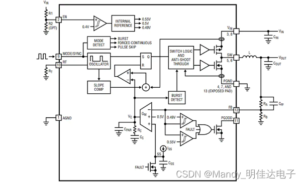
Ltc3307ahv meets EMI standard, step-down converter qca7005-al33 phy
![Jerry's watch modifies the alarm clock [chapter]](/img/d6/04fb8143027578bb707529a05db548.jpg)
Jerry's watch modifies the alarm clock [chapter]
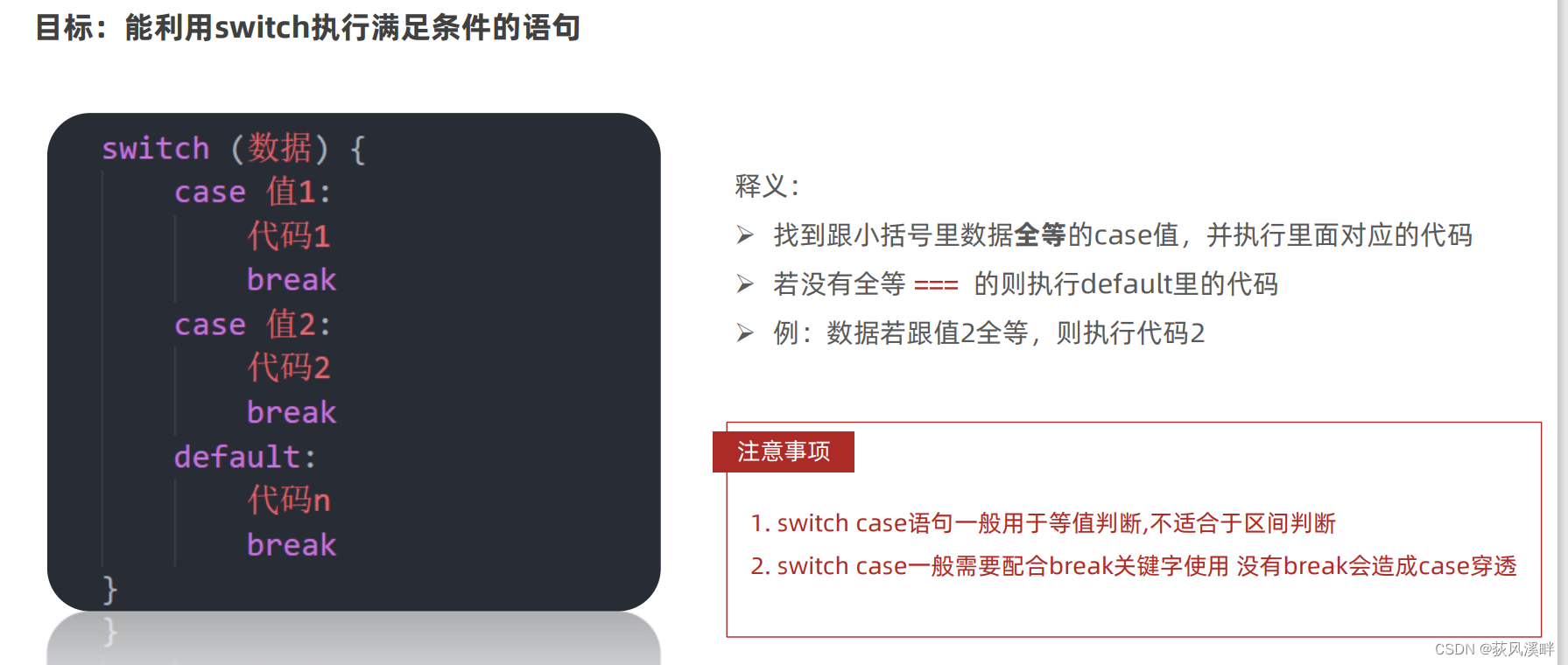
Js2day (also i++ and ++i, if statements, ternary operators, switch, while statements, for loop statements)

Linear DP acwing 895 Longest ascending subsequence

阿里发布的Redis开发文档,涵盖了所有的redis操作

PR usage skills, how to use PR to watermark?
随机推荐
ASP. Net MVC default configuration, if any, jumps to the corresponding program in the specified area
Typora+docsify quick start
PR usage skills, how to use PR to watermark?
[error record] cannot open "XXX" because Apple cannot check whether it contains malware
Browser storage scheme
Tencent three sides: in the process of writing files, the process crashes, and will the file data be lost?
模数转换器(ADC) ADE7913ARIZ 专为三相电能计量应用而设计
C operator
Uniapp develops wechat applet Tencent map function and generates sig signature of location cloud
js2day(又是i++和++i,if语句,三元运算符,switch、while语句,for循环语句)
Linear DP acwing 899 Edit distance
Linear DP acwing 898 Number triangle
8 examples of using date commands
正确遍历EntryList方法
Jerry's watch reads the alarm clock [chapter]
Get started REPORT | today, talk about the microservice architecture currently used by Tencent
Unity SKFramework框架(二十)、VFX Lab 特效库
Fully autonomous and controllable 3D cloud CAD: crowncad's convenient command search can quickly locate the specific location of the required command.
Unity skframework framework (XVI), package manager development kit Manager
About asp Net MVC project in local vs running response time is too long to access, the solution!