当前位置:网站首页>Interpretation of classic paper on model pruning: learning efficient revolutionary networks through network slimming
Interpretation of classic paper on model pruning: learning efficient revolutionary networks through network slimming
2022-07-08 02:20:00 【pogg_】
Learning Efficient Convolutional Networks through Network Slimming
Abstract :
CNN Deployment in landing , To a large extent, it is limited by its high computing cost . In this paper , The author puts forward a new CNN Learning programs :
1) Reduce model size ;
2) Reduce the occupation of model operation memory ;
3) Without affecting accuracy , Reduce the number of calculation operations .
This paper presents a simple and efficient method , It is realized through the sparsity of network channels . This method is very suitable for CNN Structure , It can minimize the cost of training , And the generated model does not need specific software and hardware to accelerate , Higher deployment performance , We call this method network pruning , It takes the heavy network as the training input model , In the process of training , Unimportant channels will be automatically screened and cut , And then generate a simplified network with considerable accuracy . We use several classic CNN Model ( Include VGGNet、ResNet and DenseNet) The feasibility of this method is verified on different image classification data sets . about VGG The Internet , The size of the model after pruning is reduced to the original 20 times , The operation is reduced to the original 5 times .
1. background :
In recent years , Convolutional neural network has become the main solution to computer vision tasks , For example, image classification 、 object detection 、 Semantic segmentation, etc . Large data sets 、 Fast growing GPU The graphics card , And new network architecture , The unprecedented large model convolutional neural network has been developed and applied . for example , from AlexNet、VGGNet and GoogLeNet To ResNet,ImageNet The classification of the challenge winning model during this period from 8 The layer develops to 100 Multi-storey .
Larger models , Although it has stronger performance , But it consumes more resources . for example ,152 layer Reset More than the 6000 All the parameters , And reasoning ( The resolution of the 224×224) when Flops More than the 20G. It's almost impossible to run on a resource constrained platform , Such as mobile terminal , Wearable devices or IOT devices .
CNN The actual deployment is mainly affected by the following :
1) The model size :CNN Powerful performance comes from its millions of trainable parameters . These parameters and network structure information are stored on disk in advance , It is loaded into memory during reasoning . for instance , stay ImageNet Store a large CNN The model will consume more than 300MB Of memory space , This is a huge burden for embedded devices that are already short of memory .
2) Run a memory : During reasoning ,CNN The parameters generated by the reasoning operation of may even occupy more memory space than the existing parameters of the model itself . This is for high-end GPU For example, the impact is slight , But for many devices with low computing power, they can't afford .
3) Amount of computation : Convolution is very computationally expensive on high-resolution images , It may take several minutes for a large model to process an image on a mobile device , This is unrealistic in practical application .
Many papers have proposed to compress large CNN The Internet ( prune ) Or direct learning is more effective CNN Model ( Distillation ) To realize the method of accelerating reasoning . It includes low rank decomposition 、 Network quantification 、 Two valued 、 Weight trim 、 Dynamic reasoning . However , Most of these methods can only solve one or two of the above problems . Besides , Some require specially designated software and hardware accelerators to speed up execution .
In this paper , We propose a simple and efficient network pruning method , It can be solved under limited resources , Deploy large CNN All the above difficulties encountered by the model .
The way to do it is :
stay BN The scaling factor in the layer is applied L1 Regularization , Reuse L1 Regularization will BN The scaling factor of the layer is constantly adjusted , Through the scaling factor, it tends to 0 To identify unimportant channel. Because each scaling factor only corresponds to a specific convolution channel ( Or neurons in the whole connective layer ), This helps to identify and prune unimportant channels in the next operation .
The effect of additional regular terms on the performance of the model is negligible , It can even help the model train with higher accuracy . Pruning unimportant channels may temporarily cause performance loss , But this effect can be achieved through subsequent finetune Amendment .
After trimming , Compared with the original network , The generated pruning network is in size 、 The running time and computing operations will be more compact .
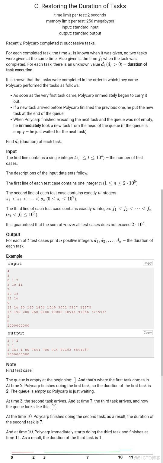
chart 1: Design scaling factor ( stay BN Reuse in layers ) In series with each channel in the convolution layer . During the training , Add sparse normalization to these scaling factors , Keep them shrinking , To identify redundant channels . The scaling factor is too small ( Orange ) The channel will be trimmed . After trimming , Will get a more compact network structure ( On the right side ), Then continue to fine tune the training , To achieve the same as the original network ( Or higher ) The accuracy of the .
Experiment on multiple datasets and different networks , It turns out that , The pruning model we obtained , Its size can be compressed to 20 times , Computing operations are reduced 5 times , At the same time , The accuracy is almost constant or even higher . Besides , The pruned model achieves reasoning acceleration on traditional hardware and software . Why? ? Because the generated model channel is narrower , There are no more redundant parameters and calculation operations .
2. Related work
In this section , We discuss five related works carried out by predecessors .
Low rank decomposition
Using singular value decomposition (SVD) And other techniques use low rank matrix to reconstruct the weight matrix in the network . This method is very effective in the full connection layer , however , because CNN The calculation operation in mainly comes from the convolution layer , therefore , Even if the model size can be compressed 3 times , But there is no obvious acceleration effect .
Weight quantization
HashNet The paper proposed to quantify the model weight . Before training , Hash the network weights into different groups , Weight values are shared in each group . Therefore, you only need to store the shared weights and their indexes , You can save a lot of storage space . The method in AlexNet and VGGNet Can be realized on 35-49 Times the compression ratio . But these technologies do not solve the problem of high computational memory , Nor can we shorten the reasoning time . Because in the process of reasoning , The shared weight needs to be restored to the original position .
《Imagenet classification using binary convolutional neural networks》 and 《Training deep
neural networks with weights and activations constrained to+1 or-1》
Convert weight into binary / Ternary weight ( The range of values is limited to {-1,1} or {-1,0,1} The weight value of ). This really saves a lot of memory , And you can also get significant acceleration . However , This extreme low bit conversion method usually brings accuracy loss .
Model pruning / sparse
《Learning both weights and connections for efficient neural network》 Propose pruning the unimportant connections of the model . Many weight values generated within the model tend to zero , Therefore, the storage space can be reduced by sparse storage . however , This method can only be accelerated by special sparse matrix operation library or hardware , And most operations are mapped by the activation function ( This part is still dense ) produce , Therefore, it is difficult to save running memory when reasoning .
Structural pruning / sparse
《 Pruning filters for efficient convnets》 Put forward , In the trained model , Trim channels with smaller weights , Then fine tune the model network to restore accuracy .《The power of sparsity in convolutional neural networks》 Propose before training , Randomly discard channel-wise The connection of , Introduce sparsity training , Although this method produces a smaller network, it also brings the loss of accuracy . Compared with these methods , We optimized the channel sparsity in the training process , Make the channel pruning process smoother , The accuracy loss is also small .《Towards compact cnns》 Introduce neuron level sparsity during training ,《 Learning structured sparsity in deep neural networks》 Propose a structured sparse learning (SSL) Methods , For sparse CNN Different structures in ( Like neurons 、 Channels or neural layers ). Both methods use the training process “ Group sparse regularization ” To get the sparsity structure of the model . Our approach does not depend on “ Group sparse regularization ”, Instead, a simple L1 Sparsity , Therefore, the optimization goal is simpler .
Because these methods are only pruning part of the network structure ( For example, neurons 、 passageway ) Not the whole weight , Therefore, they usually do not need specific libraries to speed up reasoning and ensure memory savings at runtime .
Neural architecture learning
This is an advanced method , But there are also some explorations .《Neural network architecture optimization through submodularity and supermodularity》 After determining the resources , Introduce sub module or super module optimization for network architecture search .《Neural architecture search with reinforcement learning》 and 《Designing neural network architectures using reinforcement learning》 It also proposes a method of automatically learning neural structure through reinforcement learning . The search space of these methods is very large , Therefore, hundreds of models are needed to distinguish between good and bad .
- Network pruning
We provide a scheme to realize channel thinning and pruning . In this section , We first discuss the advantages and challenges of channel sparsity , And how to use BN To effectively identify and prune unimportant channels in the network .
Advantages of channel sparsity
As discussed earlier , Sparsity can be implemented on different structures , Such as weight 、 Neuron 、 Channel or convolution . fine-grained ( Such as weight level ) The thinning of has the characteristics of high flexibility and versatility , It also has a high compression ratio , But it usually requires special software and hardware accelerators . contrary , Coarse grained layer sparseness does not require special tools to accelerate reasoning , But due to the need to trim a certain layer , Less flexibility . in fact , When the network is deep enough , Removing layers is efficient . by comparison , Channel sparsity achieves a good balance between flexibility and ease of implementation . It can be applied to any classic CNN Network or fully connected network ( Think of each neuron as a channel ), The resulting network is essentially the original network “ Streamlining ” edition , Efficient reasoning can be carried out on traditional platforms .
Challenge
To realize channel sparseness, all input and output connections related to it need to be cut off , It is difficult to prune directly on the trained model , Because the channel input / The weight of the output is unlikely to be close to zero , So we need to train while thinning . We are training well resnet Conduct channel pruning on the model , Can only reduce 10% Parameters of , But it will not cause accuracy loss .
《Learning structured sparsity in deep neural networks》 It is proposed to implement sparse regularization in the process of training objectives to solve this problem . say concretely , In the process of training , They use group lasso【1】 All filter weights corresponding to the same channel tend to 0. However , The key of this method is to correctly calculate the gradient of the additional regular term on the filter .
Scaling factor and sparsity penalty
Our idea is to introduce a scaling factor for each channel γ, Multiply by the output of this channel . Then train the network and these scaling factors , During the training process, sparse regularization is continuously applied to the scaling factor . Last , Set the scale factor value to very small ( It can even achieve 0) Cut the channel and fine tune the network again . As follows :
among (x,y) Represents the input and goal of the training ,W Represents a trainable parameter , The first item on the left indicates CNN Loss items of normal training ,g(·) Is the sparsity penalty on the scaling factor ,λ It's the balance factor , It can also be seen as normalizing the latter term . In our experiment , choice g(s)=| s |(s The absolute value of ), As L1 norm , For later sparsity training . Use the sub gradient descent method to continuously optimize the non smooth ( Unable to derive ) Of L1 Penalty item . You can also use smooth L1 Penalty replacement non smooth L1 punishment , To avoid using sub gradients at non smooth points 【2】.
Because channel pruning is equivalent to deleting the input-output connection relationship about the channel , So we can get a narrower network directly ( See the picture 1). The scaling factor plays a role in channel selection , As they optimize with the network , Unimportant channels are removed , And it will not have too much impact on generalization performance .
Use BN Scale factor in layer
BN In modern times CNN Has a wide range of applications , It can help the model converge quickly and have better generalization performance .BN The method of normalizing activation value gives us inspiration , We use it to design a simple and effective method to fuse the channel scaling factor . especially ,BN Layer using mini-batch The statistical data normalizes the activation value of the unit , We assume that zin and zout yes BN Input and output of layer ,B Represents the current mini-batch,BN The layer will perform the following transformation :
among ,µB and σB yes B The mean and standard deviation entered on ,γ and β Is a trainable affine transformation parameter ( Scale and offset ), It normalizes the activation value and linearly transforms it to any proportion .
The conventional approach is to insert a BN layer , And use channel scaling / Offset factor . therefore , We can use it directly BN Layer. γ Parameter as the scaling factor required for network pruning . Its biggest advantage is that it will not bring extra overhead to the network . in fact , This may also be the most effective way for us to try channel pruning .
1) If we are not BN Layer of CNN Add a zoom layer to the , The value of the scaling factor has no reference significance for evaluating the importance of the channel , Because both convolution layer and scaling layer are linear transformations , By reducing the value of the scaling factor , At the same time, increase the weight in the convolution layer , The results obtained remain the same .( The value of the convolution layer here is not normalized , It's still big , Even if it shrinks γ Value , The result of their mutual operation is also difficult to reduce , It is more unlikely to tend to 0)
2) If in BN Insert scale layer before layer , be BN Normalization in will completely eliminate the effect of scaling layers
3) If we were BN Insert zoom layer after layer , Then each channel has two consecutive scaling factors .
( In fact, the above three points are just to illustrate that you only need BN layer , There is no need to add additional scaling layers )
Channel pruning and fine tuning
After the channel sparseness training with regular terms , We get a lot of trends 0 Scaling factor of , Cut these channels . We use the global threshold as the proportion of channel clipping . for example , We choose 70% As a threshold , Then the scaling factor is arranged from small to large 70% Channels will be cropped . After this operation , We get a more compact network , The network has fewer parameters 、 Running takes less memory and computing operations .
More traversal ( iteration ) programme
We can also put the single ergodic learning scheme ( Sparse regularization 、 Pruning and fine tuning training ) Extend to multi traversal . In particular , Network pruning will produce a compact network , On this network , We can get a more compact model through this process again . chart 2 The dotted line of illustrates this , Experimental results show that , This multi traversal scheme will produce better results in compression .
Figure 2 : Flow chart of model pruning , Dotted lines indicate multiple iterations
Deal with cross layer connections and pre activated structures
When it is applied to design with cross layer connection and pre activation ( Such as ResNet and DenseNet) On the Internet , Some adjustments are needed . For these networks , The output of the previous layer is the input of multiple subsequent layers ,BN The layer is placed between the two ( Between the front layer and the back layer ), The sparseness of the input of the later layer ( front BN After the layer thinning operation ), It is equivalent to the subset of channels transmitted by the previous layer selectively received by the latter layer ( That is, before pruning, it was the complete collection , After pruning, it becomes a subset ). In order to obtain less parameter quantity and calculation operation in calculation , We need to place a channel selection layer to select important channels .
4、 experiment
We verify the effectiveness of our method on several data sets .
4.1 Data sets
CIFER、SVHN、ImageNet、MNIST
4.2 The Internet
stay CIFER and SVHN On dataset , We use three mainstream Networks (VGG、DenseNet40、ResNet164) The feasibility of this method is verified
stay Imagenet On , We use VGG-A Model . Because we use a lot of data to enhance , Have to get rid of dropout layer . When pruning neurons in the full connective layer , We can think of them as n individual 1×1 Convolution channel of size .
stay MNIST On dataset , We use 3 One and 《 Learning
structured sparsity in deep neural networks》 The same full connection layer .
4.3 Training 、 Pruning and fine tuning
Normal training
We train the network from scratch , All networks use SGD Algorithm
stay CIFAR and SVHN On dataset ,mini-batch=64 Respectively 160 and 20 individual epochs Training for , The initial learning rate is set as 0.1, And in 50% and 75% The training cycle is reduced 10 times .
stay ImageNet and MNIST On dataset , Let's test the model 60 and 30 individual epochs Training for ,batch size by 256, The initial learning rate is 0.1, After training 1/3 and 2/3 Stage will reduce the learning rate 10 times .
We set up weight decay=0.0001,Nesterov momentum=0.9, The channel scaling factor is initialized to 0.5, And all initialized to 1 comparison ,0.5 The initialization of is worth higher accuracy .
Sparse training
about CIFAR and SVHN Data sets , When using channel sparseness training with regular terms , Hyperparameters λ stay CIFAR-10 Set to... On the validation set 10−3, 10−4, 10−5 , This value is obtained from the grid search algorithm . about VGG, We set up λ= 10-4,Reset and DenSenet Set up λ= 10-5. stay Imagenet Upper VGG-A, We set it up λ= 10-5. Other parameter settings are consistent with normal training .
prune
When we trim the channels of the model , You need to determine the pruning threshold of the scaling factor . Set up here 40% and 60%( Table 1 ), The pruning process model keeps narrowing .
fine-tuning
After trimming , We get a narrower and more compact model , Then fine tune . stay CiFar,SVHN and Mnist On dataset , The parameter setting during fine tuning is consistent with that of normal training . stay Imagenet On dataset , We fine tune the trimmed VGG-A, The learning rate is 0.005, Because of time , We only trained 5 individual epochs.
4.4 result
CIFAR and SVHN
CIFAR and SVHN The results are shown in table 1 Shown .
Parameters and Flops The reduction of
The purpose of model pruning is to reduce the amount of calculation . The last line of each model is cropped ≥60% The passage of , At the same time, it remains the same as the original baseline Similar accuracy . The maximum number of parameters can be trimmed 90%,Flops It can usually be reduced 50%, As shown in Figure 3 .
You can see ,VGG There are a lot of redundant parameters , Pruning is very suitable . stay ResNet-164 On , Parameters and FLOP The savings are relatively small , We speculate that this is due to its “bottleneck” The structure has played the role of selecting channels . Besides , stay CiFar-100 On , The cutting rate is usually slightly lower than CiFar-10 and SVHN, This may be due to CiFar-100 Reasons for including more classes .
Regularization effect
From the table 1 in , We can observe that , stay Reset and DenSenet On , Usually in pruning 40% Channel time , Fine tuning the network can achieve lower classification error than the original model . Such as after 40% Channel trimmed DenseNet-40 stay CIFAR-10 The test error on is 5.19%, Almost lower than the original model 1%. We assume that this is due to L1 The effect of sparse regularization on channels , It provides feature selection of network middle layer . We will analyze this effect in the next section .
ImageNet
ImageNet The results of the dataset are shown in table 2 in . When deleted 50% When you're in the middle of the tunnel , Parameter quantity prunable super 5 times , and FLOP Can reduce 30.4%. It could be because VGG-A Among the convolution layers involved in intensive computation 378 individual (2752 individual ) Channels are trimmed , In the full connection layer with dense parameters 5094 Neurons (8192 individual ) Be pruned . Here's the thing to watch ,ImageNet-1000 On dataset , Our method realizes clipping without losing accuracy , More efficient than other pruning methods .
MNIST
stay MNIST On dataset , Use our method with structured sparse learning (SSL) Methods for comparison , The results are shown in Table 3 , Although our method is mainly used to trim convolution channels , But it can also prune neurons in the whole connective layer well . In this experiment , We observed that when setting the global threshold for pruning , It is possible to completely delete a certain layer , So we only trim each layer 80% Of neurons . While trimming more parameters , The test error remains low , Obviously better than 《 Learning
structured sparsity in deep neural networks》 Proposed method .
4.5 The result of multiple iterations
We use VGG stay CiFar Multiple iterations on the dataset , The test results are shown in Table 4 ,VGG stay CIFAR-10 and CIFAR100 The test errors are 6.34% and 26.74%.“Trained” and “Fine-tuned” It represents the test error of the sparsity training model and the fine-tuning pruning model respectively (%). Parameters and FLOP Trim ratio , Corresponds to the ratio between the model in this row and the model in the next row .
5 analysis
In this section, we analyze two superparameters : Trim percentage ( Global threshold )t And regularization terms λ The important impact of
Effect of trim percentage
Once we get a model trained by sparse regularization , We can decide how many channels to delete from the model . If we cut too few channels , The resources saved will be very limited . however , If you trim too many channels , May destroy the model , And the accuracy cannot be restored by fine tuning . We trained a λ=10-5 Of DenseNet40 Model , To show the effect of trimming different percentage channels . The results are summarized in Figure 5 in
Only when the threshold exceeds 80% when , The fine-tuning model will be worse than the baseline model . It is worth noting that , When training with sparsity , Even without fine tuning , This model also performs better than the original model . This may be due to L1 Sparsity has a good effect on the channel scaling factor .
Influence of channel sparse regularization
L1 The purpose of the sparse term is to force many scaling factors close to zero . In the figure 4 in , We use different λ Value plots the distribution of scaling factors across the network . And in this experiment , We use VGG stay CiFar-10 Training on data sets .
Can be observed , With λ An increase in , The scaling factor is increasingly concentrated around zero . When λ=0 when , No sparse regularization , The distribution is relatively flat . When λ=10−4 when , Almost all scaling factors fall into a small area close to zero . This process can be seen as feature selection occurring in deep Networks , That is, only select important channels . We went further through Heatmap Visualize this process . chart 6 Shows that during training ,VGG The size of the scaling factor of a layer . Each channel starts with the same initialization weight ; With training , The scaling factor of some channels becomes larger ( Brighter ), The scaling factor of some channels becomes smaller and smaller ( Darker ).
6. summary
We propose network slimming technology to learn more compact CNN. It's direct to BN The scaling factor in the layer imposes the regularization of the sparse factor , Thus, unimportant channels can be automatically identified during training , Then trim . On multiple data sets , We have proven that , The proposed method can significantly reduce the computing cost of the network ( the height is 20×), No loss of accuracy . what's more , The proposed method reduces the size of the model at the same time 、 Run memory and computing operations , At the same time, it introduces the minimum computational cost for the training process , And the generated model does not need special libraries / Hardware to reason .
Add :
BN Calculation formula :
【1】 What is? group lasso:https://blog.csdn.net/hestendelin/article/details/101546489
【2】sub-gradient:https://blog.csdn.net/qq_32742009/article/details/81704139
【3】 What is low rank decomposition :
Low rank matrices : If X It's a m That's ok n The numerical matrix of the column ,rank(X) yes X The rank of , If rank (X) Far less than m and n, Then we call X It's a low rank matrix . Each row or column of a low rank matrix can be expressed linearly with other rows or columns , It can be seen that it contains a lot of redundant information . Take advantage of this redundant information , Missing data can be recovered , You can also extract features from the data .
Low rank decomposition :
Method : Using two K1 Replace one with the convolution kernel of KK Convolution kernel (decompose the K convolutions into two separable convolutions of size 1 × K and K × 1)
principle : Weight vectors are mainly distributed in some low rank subspaces , Use a few bases to reconstruct the weight matrix
Replace the original matrix with a low rank matrix , The number of parameters can be reduced , This reduces the amount of calculation .
Purpose : Remove redundancy , And reduce the weight parameters
【4】Grid Search:https://www.cnblogs.com/ysugyl/p/8711205.html

边栏推荐
- Applet running under the framework of fluent 3.0
- Keras深度学习实战——基于Inception v3实现性别分类
- How to use diffusion models for interpolation—— Principle analysis and code practice
- Semantic segmentation | learning record (3) FCN
- leetcode 865. Smallest Subtree with all the Deepest Nodes | 865.具有所有最深节点的最小子树(树的BFS,parent反向索引map)
- The bank needs to build the middle office capability of the intelligent customer service module to drive the upgrade of the whole scene intelligent customer service
- For friends who are not fat at all, nature tells you the reason: it is a genetic mutation
- 很多小夥伴不太了解ORM框架的底層原理,這不,冰河帶你10分鐘手擼一個極簡版ORM框架(趕快收藏吧)
- Height of life
- leetcode 866. Prime Palindrome | 866. prime palindromes
猜你喜欢
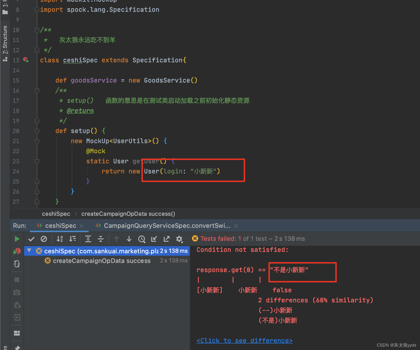
Spock单元测试框架介绍及在美团优选的实践_第二章(static静态方法mock方式)
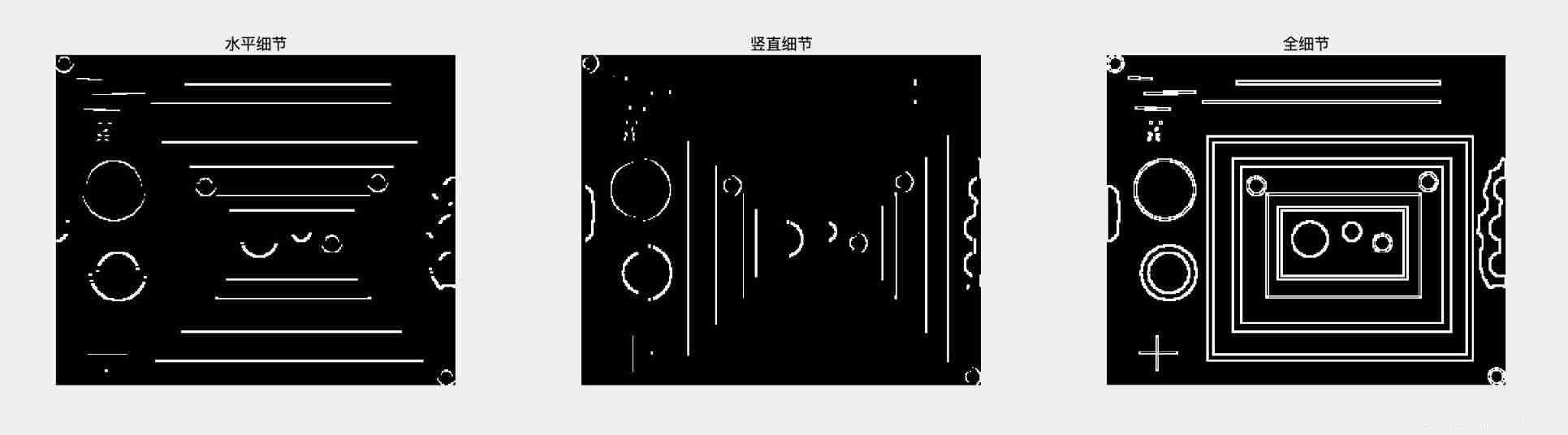
image enhancement

分布式定时任务之XXL-JOB

What are the types of system tests? Let me introduce them to you

银行需要搭建智能客服模块的中台能力,驱动全场景智能客服务升级
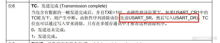
关于TXE和TC标志位的小知识

leetcode 865. Smallest Subtree with all the Deepest Nodes | 865. The smallest subtree with all the deepest nodes (BFs of the tree, parent reverse index map)

leetcode 869. Reordered Power of 2 | 869. 重新排序得到 2 的幂(状态压缩)
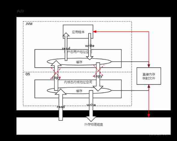
JVM memory and garbage collection-3-direct memory
#797div3 A---C
随机推荐
Yolo fast+dnn+flask realizes streaming and streaming on mobile terminals and displays them on the web
生命的高度
leetcode 866. Prime Palindrome | 866. 回文素数
Le chemin du poisson et des crevettes
Master go game through deep neural network and tree search
Ml self realization / logistic regression / binary classification
Leetcode question brushing record | 283_ Move zero
What are the types of system tests? Let me introduce them to you
Keras深度学习实战——基于Inception v3实现性别分类
线程死锁——死锁产生的条件
Kwai applet guaranteed payment PHP source code packaging
Redismission source code analysis
Introduction to Microsoft ad super Foundation
"Hands on learning in depth" Chapter 2 - preparatory knowledge_ 2.1 data operation_ Learning thinking and exercise answers
[knowledge map] interpretable recommendation based on knowledge map through deep reinforcement learning
Force buckle 5_ 876. Intermediate node of linked list
Semantic segmentation | learning record (4) expansion convolution (void convolution)
metasploit
CorelDRAW2022下载安装电脑系统要求技术规格
魚和蝦走的路