当前位置:网站首页>Key review route of probability theory and mathematical statistics examination
Key review route of probability theory and mathematical statistics examination
2022-07-05 04:23:00 【IOT classmate Huang】
The key review route of probability theory and mathematical statistics exam
List of articles
Preface
Hope to pass a simple route , Achieve accurate and efficient preparation for tomorrow's exam . Don't talk much , To rush !
The content is divided into two parts: probability theory and mathematical statistics , The middle series is the law of large numbers and central limit theorem in Chapter 5 .
MindMap
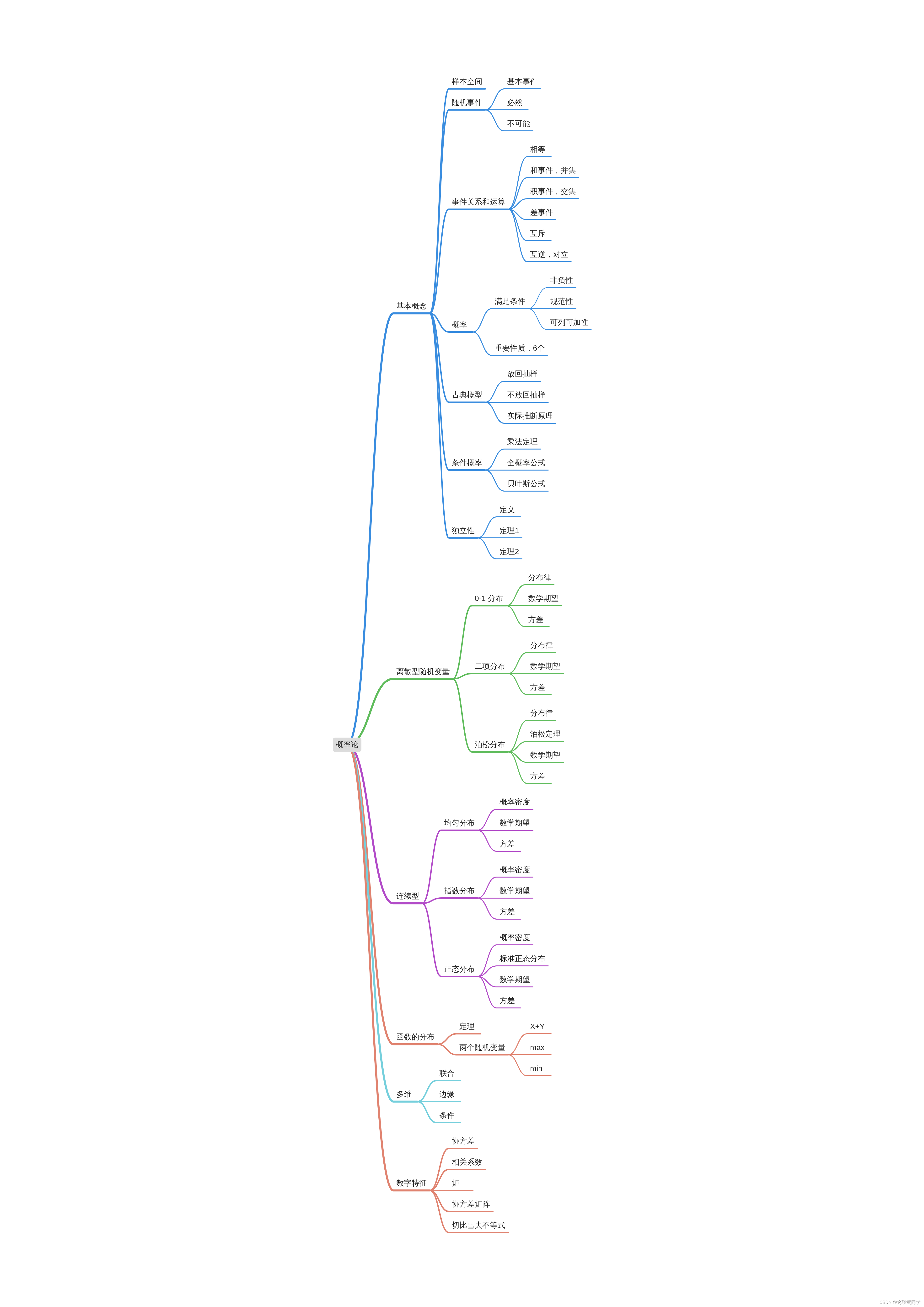
Probability theory part
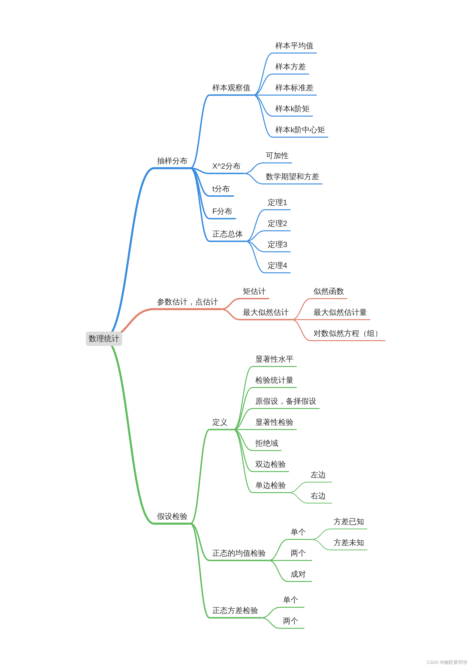
Mathematical statistics
probability theory
Basic concepts
The content of this part , My suggestion is to look directly at my previous blog, Or reading books and other online classes ppt And so on. .
I won't enumerate the distribution function of random variables , You can deduce it directly through the distribution law or probability density
discrete
0-1 Distribution
X~b§
Distribution law
P { X = k } = p k ( 1 − p ) 1 − k , k = 1 , 0 P\{X=k \} = p^k(1-p)^{1-k}, \qquad k = 1, 0 P{ X=k}=pk(1−p)1−k,k=1,0
| X | 0 | 1 |
|---|---|---|
| p_k | 1-p | p |
Mathematical expectation
E ( X ) = p E(X) = p E(X)=p
variance
D ( X ) = ( 1 − p ) ⋅ p D(X) = (1-p)\cdot p D(X)=(1−p)⋅p
The binomial distribution
X~b(n, p)
Distribution law
P { X = k } = p k ( 1 − p ) 1 − k P\{X=k \} = p^k(1-p)^{1-k} P{ X=k}=pk(1−p)1−k
Mathematical expectation
E ( X ) = n p E(X) = np E(X)=np
variance
D ( X ) = n ( 1 − p ) ⋅ p D(X) = n(1-p)\cdot p D(X)=n(1−p)⋅p
Poisson distribution
X~π(λ)
Distribution law
P { X = k } = λ k e − λ k ! , k = 0 , 1 , 2... P\{X=k \} = \frac{\lambda^ke^{-\lambda}}{k!}, \qquad k=0,1,2... P{ X=k}=k!λke−λ,k=0,1,2...
Poisson's theorem
Is to use Poisson to approximate binomial ,np=λ
lim n → ∞ C n k ( 1 − p n ) n − k = λ k e − λ k ! \lim_{n\rightarrow \infty}{C_n^k(1-p_n)^{n-k}} = \frac{\lambda^ke^{-\lambda}}{k!} n→∞limCnk(1−pn)n−k=k!λke−λ
Mathematical expectation
E ( X ) = λ E(X) = \lambda E(X)=λ
variance
D ( X ) = λ D(X) = \lambda D(X)=λ
Continuous type
Uniform distribution
X~U(a, b)
Probability density
KaTeX parse error: No such environment: align at position 26: …eft \{ \begin{̲a̲l̲i̲g̲n̲}̲ &\frac{1}{b…
expect
E ( X ) = a + b 2 E(X) = \frac {a+b}{2} E(X)=2a+b
variance
D ( X ) = ( b − a ) 2 12 D(X) = \frac{(b-a)^2}{12} D(X)=12(b−a)2
An index distribution
X~E(θ)
Probability density
KaTeX parse error: No such environment: align at position 26: …eft \{ \begin{̲a̲l̲i̲g̲n̲}̲ &\frac{1}{\…
expect
E ( X ) = θ E(X) = \theta E(X)=θ
variance
D ( X ) = θ 2 D(X) = \theta^2 D(X)=θ2
Normal distribution
X~N(μ, σ)
Probability density
f ( x ) = 1 2 π σ e − ( x − u ) 2 2 σ 2 , − ∞ < x < ∞ f(x) = \frac{1}{\sqrt{2\pi}\sigma}e^{-\frac{(x-u)^2}{2\sigma^2}}, \qquad -\infty < x < \infty f(x)=2πσ1e−2σ2(x−u)2,−∞<x<∞
Standard normal distribution
X ∼ N ( 0 , 1 2 ) φ ( x ) = 1 2 π e − x 2 / 2 X\sim N(0, 1^2)\\ \varphi(x) = \frac{1}{\sqrt{2\pi}}e^{-x^2/2} X∼N(0,12)φ(x)=2π1e−x2/2
Expectation and variance , In general, as long as it is converted into a standard normal distribution , Then it can be solved with the variance and expectation of the standard normal distribution .
expect
E ( x ) = μ E(x) = \mu E(x)=μ
variance
D ( X ) = σ 2 D(X) = \sigma^2 D(X)=σ2
In addition to these, there are actually random variable functions in probability theory , Multi dimensional edges and conditions and combinations , There are also covariance and moments in Chapter 4 . But I won't mention these contents , If necessary, you can see blog Or textbooks .
mathematical statistics
It's swinging , Look at this directly . I'm going back to bed .
边栏推荐
- All in one 1413: determine base
- Threejs Internet of things, 3D visualization of factory
- OWASP top 10 vulnerability Guide (2021)
- 【虛幻引擎UE】實現UE5像素流部署僅需六步操作少走彎路!(4.26和4.27原理類似)
- MacBook安装postgreSQL+postgis
- Three level linkage demo of uniapp uview u-picker components
- User behavior collection platform
- Looking back on 2021, looking forward to 2022 | a year between CSDN and me
- Burpsuite grabs app packets
- 小程序中实现文章的关注功能
猜你喜欢
![[uniapp] system hot update implementation ideas](/img/1e/77ee9d9f0e08fa2a7734a54e0c5020.png)
[uniapp] system hot update implementation ideas
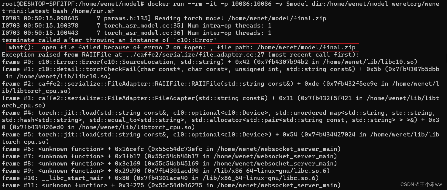
WeNet:面向工业落地的E2E语音识别工具

如何实现实时音视频聊天功能

Common features of ES6
![[phantom engine UE] package error appears! Solutions to findpin errors](/img/d5/6747e20da6a8a4ca461094bd27bbf0.png)
[phantom engine UE] package error appears! Solutions to findpin errors
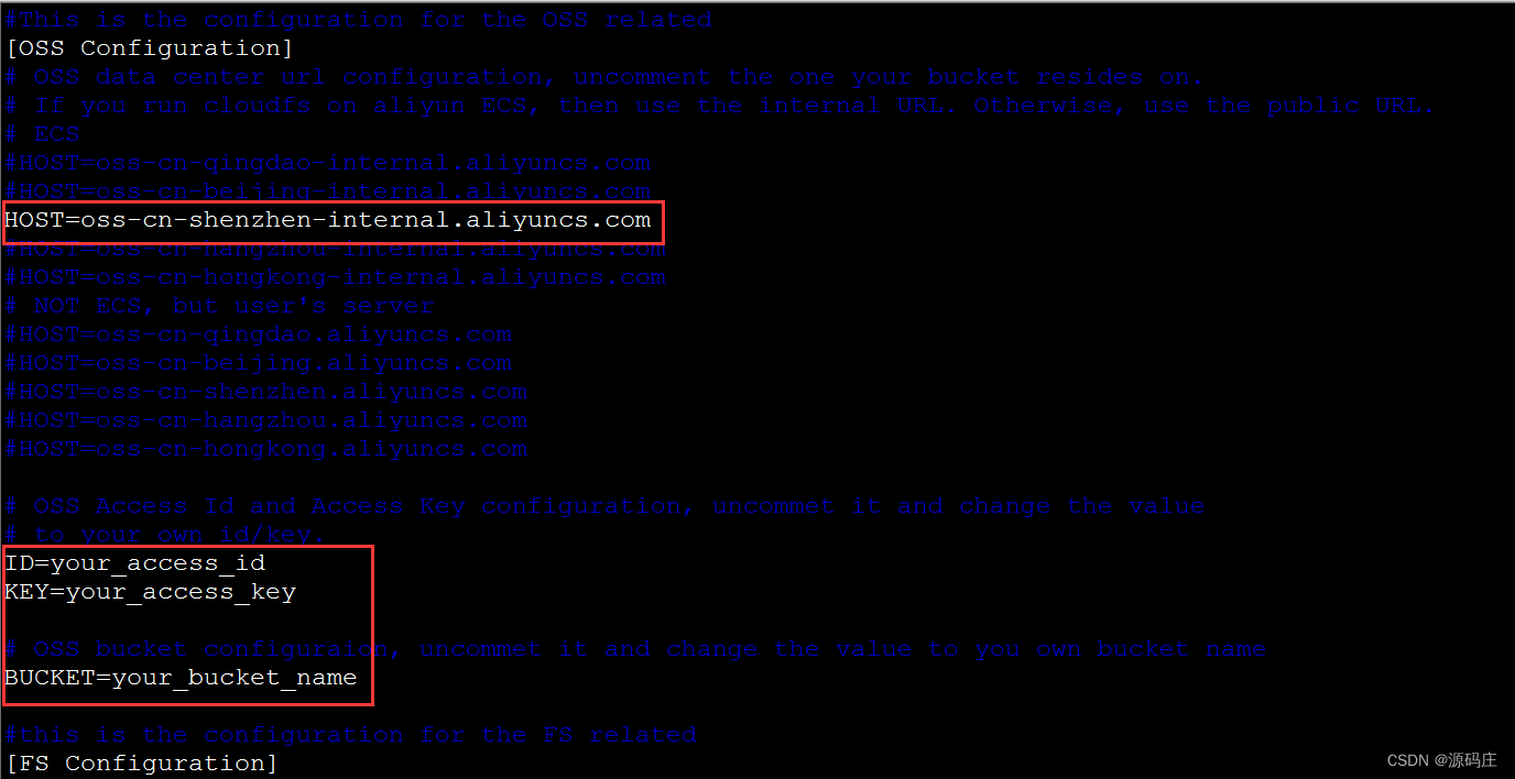
Alibaba cloud ECS uses cloudfs4oss to mount OSS

Three level linkage demo of uniapp uview u-picker components
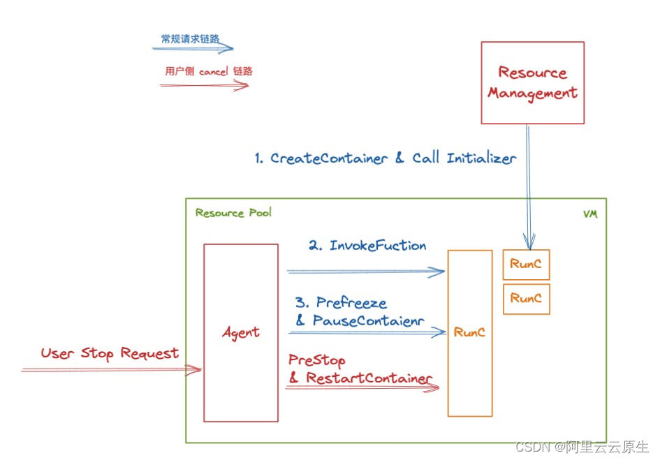
解密函数计算异步任务能力之「任务的状态及生命周期管理」

C26451: arithmetic overflow: use the operator * on a 4-byte value, and then convert the result to an 8-byte value. To avoid overflow, cast the value to wide type before calling the operator * (io.2)
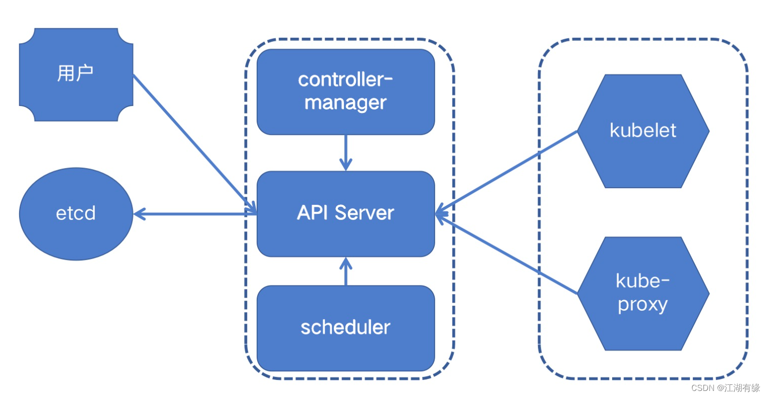
Scheduling system of kubernetes cluster
随机推荐
快手、抖音、视频号交战内容付费
[uniapp] system hot update implementation ideas
函数(基本:参数,返回值)
Web开发人员应该养成的10个编程习惯
Fuel consumption calculator
Threejs realizes rain, snow, overcast, sunny, flame
Bit operation skills
线上故障突突突?如何紧急诊断、排查与恢复
Alibaba cloud ECS uses cloudfs4oss to mount OSS
Realize the attention function of the article in the applet
Rust blockchain development - signature encryption and private key public key
[untitled]
指针函数(基础)
Open graph protocol
【虚幻引擎UE】实现UE5像素流部署仅需六步操作少走弯路!(4.26和4.27原理类似)
How to carry out "small step reconstruction"?
How to solve the problem that easycvr changes the recording storage path and does not generate recording files?
The development of mobile IM based on TCP still needs to keep the heartbeat alive
mysql的七种join连接查询
Threejs Internet of things, 3D visualization of factory