当前位置:网站首页>Outlier detection technology of time series data
Outlier detection technology of time series data
2022-07-07 07:21:00 【Data analysis cases】
author | Cookies
01 summary
Usually, the outliers of time series data are mainly divided into three categories :

02 Common features of time series data
Common characteristics of time series data
features | describe |
cycle ( frequency ) | The data is repeated |
trend | The data shows an increase 、 Downward trend |
Seasonality | Repetitive and predictable changes on a trend line in a year or less |
Autocorrelation | Represents the dependency between data |
nonlinear | Time series contain complex data sets represented by nonlinear models |
skewness | Measure symmetry , Or more specifically , Lack of symmetry |
kurtosis | If the data peaks or flattens relative to the normal distribution , Then take measures |
Hillock in the forest | Measure the long-term memory of time series |
Lyapunov exponent | Measure the divergence speed of nearby tracks |
Common indicators for modeling experiments , Measure the quality of the model
indicators | describe |
Bias | The arithmetic mean of the error |
MAD | Mean absolute deviation , Also known as MAE |
MAPE | Mean absolute percentage error |
MSE | Mean square of error |
SAE | The sum of absolute errors |
ME | Average error |
MASE | Mean absolute proportional error |
MPE | Average percentage error |
03 Anomaly detection methods
There are three main categories :
- Statistical model based outlier detection technology based on statistical model builds all data into a data model , It believes that outliers are objects that cannot fit perfectly with the model .
- Based on proximity, it is usually possible to define proximity measures between objects . Exception objects are objects that are far away from most other objects .
- The density estimation of technical objects based on density can be calculated relatively directly , Especially when there are proximity measures between objects . When the local density of a point is significantly lower than most of its neighbors , May be considered abnormal .
Outlier detection based on statistical model
Data based , Build a probability distribution model , Get the module Probability density function of type . Usually , The probability of outliers is very low .
Univariate outlier detection based on Chint distribution

Outlier detection of multivariate normal distribution
For multivariate Gaussian distribution detection , We want to use a method similar to univariate Gaussian distribution . for example , If the point has a low probability about the estimated data , Then classify them as outliers .
In fact, Mahalanobis distance is also a statistical algorithm , Point to base distribution Mahalanobis The distance is directly related to the probability of the point
in summary , Two outlier detection methods based on statistical model , Statistical techniques based on standards are needed ( Such as distribution Estimation of parameters ) above . Such methods may be effective for low dimensional data , But for high-dimensional data , The data distribution is very complex , The detection effect based on statistical model will be poor .
Outlier detection based on proximity
Markov distance

It's easy to prove : Point to data mean Mahalanobis The distance is directly related to the probability of the point , Equal to the logarithm of the probability density of the point plus a constant . therefore , It can be done to Mahalanobis Sort by distance , Large distance , It can be regarded as an outlier .
KNN

Density based outlier detection
From a density based point of view , Outliers are objects in low-density areas .
There are three ways to define density .
Inverse distance
The density of an object is around the object k The reciprocal of the average distance of the nearest neighbors .


radius d Number of in
That is, the density around an object is equal to the specified radius of the object d Number of objects in .d It's human choice , So this d Your choice is very important .
Relative density
Ready to use x And its nearest neighbor y The ratio of the average density to the relative density .


Independent forest Isolation Forest
First , To understand the independent forest , You must understand what an independent tree is , Hereinafter referred to as" iTree .iTree It's a random two Fork tree , Each node has either two child nodes ( They are called left subtree and right subtree ), Or there are no child nodes ( It's called a leaf node ). Given data set D, here D All properties of are continuous variables , iTree The composition of the system is as follows :
- Randomly select an attribute A.
- Randomly select a value of this property value .
- according to A Classify each record , hold A Less than value The record of is placed on the left subtree , Put greater than or equal to value The records of are placed on the right subtree .
- Recursively construct left subtree and right subtree , Until the conditions are met :① The incoming data set has only one or more identical records ;② The height of the tree has reached the height width value .
iTree After construction , Next, predict the data . The process of prediction is to record the test from iTree The root node starts searching , Determine which leaf node the test record falls on .iTree The hypothesis that can detect anomalies is : The outliers are usually very rare , stay iTree Will soon be assigned to leaf nodes . in other words , stay iTree in , Outliers are generally represented by the path from the leaf node to the root node h(x) Very short . therefore , It can be used h(x) To determine whether a record belongs to an outlier .

There are also points to note in the implementation :
- Random trees are unstable , But put more trees iTree Combine , formation iForest It becomes strong
- structure iForest The method is similar to the method of constructing random forest , Are randomly sampling a part of the data set to construct each tree , Ensure the difference between different trees . But the difference is , We need to limit the sample size . The normal value and abnormal value overlap before sampling , After sampling, normal value and abnormal value can be effectively distinguished .

- Need to limit iTree The maximum height of , Because there are few abnormal value records , Its path length is also relatively small . The tree is too deep, increasing meaningless computational consumption .
in summary , Independent forest is essentially an unsupervised algorithm , Class labels that do not require a priori . When dealing with high-dimensional data , Not all attributes are used , But through kurtosis coefficient ( Low kurtosis , The long tail is too long , It's hard to judge the abnormality ; High kurtosis , Then most data sets , Convenient judgment ) Pick some valuable attributes , And then we can move on iForest Construction , The effect of the algorithm will be better .
The darker the color, the higher the abnormal value , The lighter the color, the lower the abnormal value . It can be seen that , The prediction effect of the model is good , Color distribution law and test and outlier The data set exactly matches .

04 Industry practice
Common open source anomaly monitoring systems


边栏推荐
- Composition API premise
- JS decorator @decorator learning notes
- 1090: integer power (multi instance test)
- AVL树的实现
- main函数在import语句中的特殊行为
- . Net core accesses uncommon static file types (MIME types)
- Precise space-time travel flow regulation system - ultra-high precision positioning system based on UWB
- A slow SQL drags the whole system down
- FPGA course: application scenario of jesd204b (dry goods sharing)
- . Net 5 fluentftp connection FTP failure problem: this operation is only allowed using a successfully authenticated context
猜你喜欢
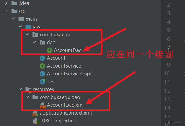
Bindingexception exception (error reporting) processing
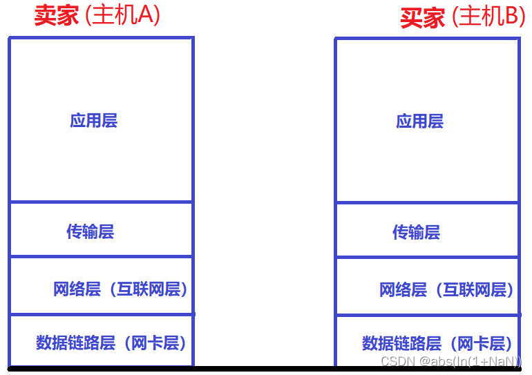
Basic process of network transmission using tcp/ip four layer model
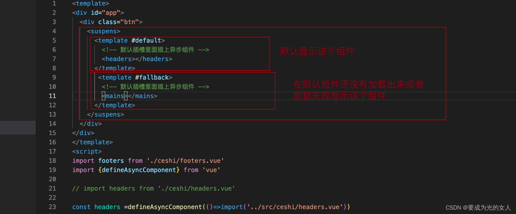
异步组件和Suspense(真实开发中)

Unity3d learning notes
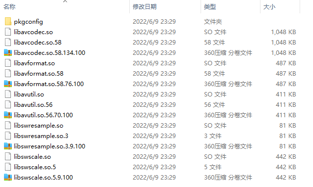
mips uclibc 交叉编译ffmpeg,支持 G711A 编解码

Sqlmap tutorial (IV) practical skills three: bypass the firewall
LC interview question 02.07 Linked list intersection & lc142 Circular linked list II
Four goals for the construction of intelligent safety risk management and control platform for hazardous chemical enterprises in Chemical Industry Park

Composition API 前提
AVL树的实现
随机推荐
2018 Jiangsu Vocational College skills competition vocational group "information security management and evaluation" competition assignment
Bus message bus
抽絲剝繭C語言(高階)指針的進階
Kuboard can't send email and nail alarm problem is solved
LC 面试题 02.07. 链表相交 & LC142. 环形链表II
软件验收测试
Academic report series (VI) - autonomous driving on the journey to full autonomy
Network foundation - header, encapsulation and unpacking
Cloud backup project
Introduction to abnova's in vitro mRNA transcription workflow and capping method
FullGC问题分析及解决办法总结
Lvs+kept (DR mode) learning notes
Esxi attaching mobile (Mechanical) hard disk detailed tutorial
Leetcode t1165: log analysis
我理想的软件测试人员发展状态
A slow SQL drags the whole system down
组件的嵌套和拆分
Special behavior of main function in import statement
Détailler le bleu dans les tâches de traduction automatique
How to model and simulate the target robot [mathematical / control significance]