当前位置:网站首页>A Cooperative Approach to Particle Swarm Optimization
A Cooperative Approach to Particle Swarm Optimization
2022-07-06 01:24:00 【Figure throne】
0、 Background
CPSO It's based on standards PSO Deformed from , This paper presents a new method of PSO Variants of the algorithm , Called collaborative particle swarm optimizer , or CPSO. Using cooperative behavior to significantly improve the performance of the original algorithm , This is achieved by using multiple groups to jointly optimize the different components of the solution vector .
Van den Bergh F, Engelbrecht A P. A cooperative approach to particle swarm optimization[J]. IEEE transactions on evolutionary computation, 2004, 8(3): 225-239.

1、CPSO
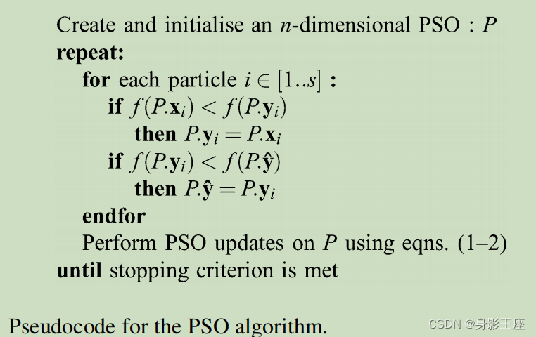
1.1 standard PSO
of PSO Algorithm and specific implementation , See my previous blog : standard PSO.
Speed update formula :
![\begin{aligned} v_{i, j}(t+1)=w v_{i, j}(t)+c_{1} r_{1, i}(t) & {\left[y_{i, j}(t)-x_{i, j}(t)\right] } +c_{2} r_{2, i}(t)\left[\hat{y}_{j}(t)-x_{i, j}(t)\right] &(1)\end{aligned}](http://img.inotgo.com/imagesLocal/202207/06/202207060119162576_7.gif)
Position update formula :

pbest Update formula :

gbest Update formula :

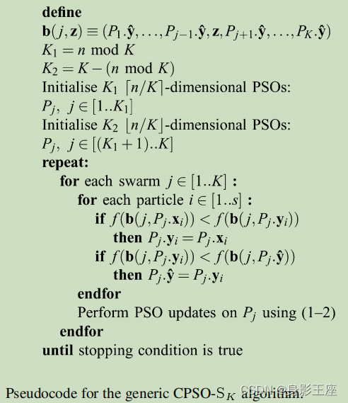
1.2 CPSO_Sk
CPSO The algorithm decomposes the larger search space into several smaller spaces , Therefore, each subgroup converges to the solution contained in its subspace significantly faster than the standard PSO In primitive n Convergence rate on dimensional search space .
If each subspace dimension is set to 1 dimension , So the whole n Dimensional space is divided into n individual 1 The subspace of dimension .

-
 It means s*1 Dimensional sample subspace ,s Represents the total number of particles ,1 representative n One dimensional variable in dimension .
  On behalf of the j In the subspace i The position of a particle .
 On behalf of the j In the subspace i Of particles pbest.
 On behalf of the j Subspace gbest.
 This function returns a n Dimension vector , By connecting all the global best vectors of all subspaces , Except for j Weight , It is replaced by z.
 It means s*1 Dimensional sample subspace ,s Represents the total number of particles ,1 representative n One dimensional variable in dimension .
 On behalf of the j In the subspace i The position of a particle .
 On behalf of the j In the subspace i Of particles pbest.
 On behalf of the j Subspace gbest.
 This function returns a n Dimension vector , By connecting all the global best vectors of all subspaces , Except for j Weight , It is replaced by z.
 If each subspace dimension is set to k dimension , So the whole n Dimensional space is divided into  individual k The subspace of dimension .
1.3 CPSO_Hk
In the previous section ,CPSO_Sk The algorithm is easy to fall into the local optimal position of subspace , Global search capability compared to PSO Declined . In order to improve the CPSO_Sk Global search capability , take CPSO_Sk and PSO Combine , To form the CPSO_Hk Algorithm .
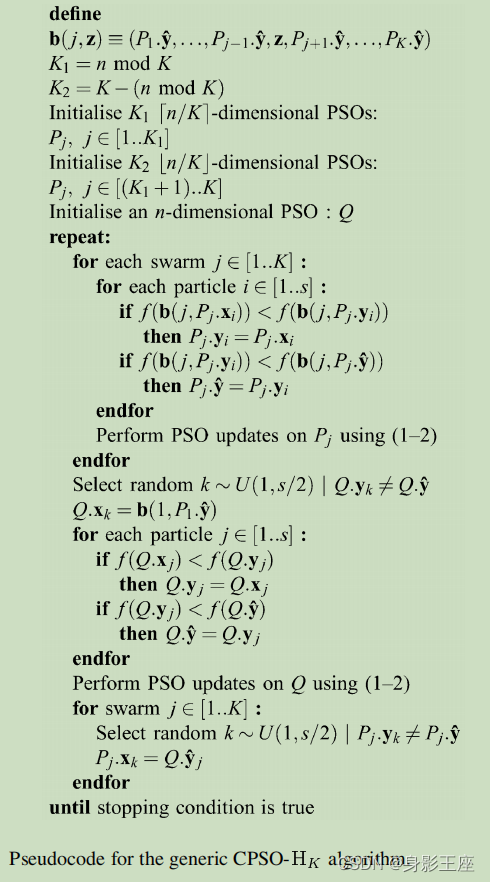
- P and Q The total number of populations is s, here P and Q The population number of is set to s/2.
- k Is a sample of a randomly selected population , And carry on Q and P The corresponding information interaction between populations .
1.4 Algorithm reproduction and experiment
The algorithm experiment in this article is complex , I don't intend to reproduce it according to the ideas in the article . Here I reproduce the algorithm and carry out simple experiments , See if there are any effects , If effective, it is convenient to apply its ideas to other places . Therefore, the recurrence of this article only stays in the understanding and reference of thought .
PSO( Repeat the experiment 100 Time , Average. ):
function f = Rastrigin(x)
% the Rastrigin function
% xi = [-5.12,5.12]
d = size(x,2);
f = 10*d + sum(x.^2 - 10*cos(2*pi*x),2);
end
clc;clear;clearvars;
% Random generation 5 Data
num_initial = 20;
num_vari = 60;
% Search range
upper_bound = 5.12;
lower_bound = -5.12;
iter = 12000;
w = 1;
% Random generation 5 Data , And obtain its evaluation value
sample_x = lhsdesign(num_initial, num_vari).*(upper_bound - lower_bound) + lower_bound.*ones(num_initial, num_vari);
sample_y = Rastrigin(sample_x);
Fmin = zeros(iter, 1);
aver_Fmin = zeros(iter, 1);
for n = 1 : 100
k = 1;
% Initialize some parameters
pbestx = sample_x;
pbesty = sample_y;
% Current location information presentx
presentx = lhsdesign(num_initial, num_vari).*(upper_bound - lower_bound) + lower_bound.*ones(num_initial, num_vari);
vx = sample_x;
[fmin, gbest] = min(pbesty);
fprintf("n: %.4f\n", n);
% fprintf("iter 0 fmin: %.4f\n", fmin);
for i = 1 : iter
r = rand(num_initial, num_vari);
% pso Update the location of the next step , Here you can set the boundary if it exceeds the search range
vx = w.*vx + 2 * r .* (pbestx - presentx) + 2 * r .* (pbestx(gbest, :) - presentx);
vx(vx > upper_bound) = upper_bound;
vx(vx < lower_bound) = lower_bound;
presentx = presentx + vx;
presentx(presentx > upper_bound) = upper_bound;
presentx(presentx < lower_bound) = lower_bound;
presenty = Rastrigin(presentx);
% Update the best location for each individual
pbestx(presenty < pbesty, :) = presentx(presenty < pbesty, :);
pbesty(presenty < pbesty, :) = presenty(presenty < pbesty, :);
% Update the best location of all individuals
[fmin, gbest] = min(pbesty);
% fprintf("iter %d fmin: %.4f\n", i, fmin);
Fmin(k, 1) = fmin;
k = k +1;
end
aver_Fmin = aver_Fmin + Fmin;
end
aver_Fmin = aver_Fmin ./ 100;
% disp(pbestx(gbest, :));
plot(aver_Fmin);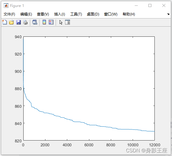
CPSO_Sk( Repeat the experiment 100 Time , Average. ):
clc;clear;clearvars;
%  Random generation 20 Data
num_initial = 20;
num_vari = 60;
%  Search range
upper_bound = 5.12;
lower_bound = -5.12;
%  Calculate during iteration y Total number of values
eval_num = 12000;
% K Represents the number of partitioned subspaces ,sub_num Represents the dimension of each subspace
K = 5;
sub_num = num_vari / K;
%  The number of iterations of the algorithm
iter = eval_num / K;
w = 1;
%  Random generation 20 Data , And obtain its evaluation value
sample_x = lhsdesign(num_initial, num_vari).*(upper_bound - lower_bound) + lower_bound.*ones(num_initial, num_vari);
sample_y = Rastrigin(sample_x);
Fmin = zeros(eval_num, 1);
aver_Fmin = zeros(eval_num, 1);

for n = 1 : 100
    n1 = 1;
    %  Initialize some parameters
    pbestx = sample_x;
    pbesty = sample_y;
    %  Current location information presentx
    presentx = lhsdesign(num_initial, num_vari).*(upper_bound - lower_bound) + lower_bound.*ones(num_initial, num_vari);
    vx = sample_x;
    [fmin, gbest] = min(pbesty);
    global_best_x = pbestx(gbest, :);
    fprintf("n: %.4f\n", n);
    % fprintf("iter 0 fmin: %.4f\n", fmin);
    for i = 1 : iter
        for i1 = 1 : K
            ind = ((1 + (i1 - 1) * sub_num) : i1 * sub_num);
            r = rand(num_initial, sub_num);
            % pso Update the location of the next step , Here you can set the boundary if it exceeds the search range
            vx(:, ind) = w.*vx(:, ind) + 2 * r .* (pbestx(:, ind) - presentx(:, ind)) + 2 * r .* (pbestx(gbest, ind) - presentx(:, ind));
            vx1 = vx(:, ind);
            vx1(vx1 > upper_bound) = upper_bound;
            vx1(vx1 < lower_bound) = lower_bound;
            vx(:, ind) = vx1;
            presentx(:, ind) = presentx(:, ind) + vx1;
            presentx1 = presentx(:, ind);
            presentx1(presentx1 > upper_bound) = upper_bound;
            presentx1(presentx1 < lower_bound) = lower_bound;
            presentx(:, ind) = presentx1;

            presentx2 = repmat(global_best_x, num_initial, 1);
            presentx2(:, ind) = presentx1;
            presenty = Rastrigin(presentx2);

            %  Update the best location for each individual
            pbestx1 = pbestx(:, ind);
            pbestx1(presenty < pbesty, :) = presentx1(presenty < pbesty, :);
            pbestx(:, ind) = pbestx1;
            pbesty(presenty < pbesty, :) = presenty(presenty < pbesty, :);

            %  Update the best location of all individuals
            [fmin, gbest] = min(pbesty);
            global_best_x = pbestx(gbest, :);
            Fmin(n1, 1) = fmin;
            n1 = n1 +1;
            % fprintf("iter %d fmin: %.4f\n", i, fmin);
        end
    end
    aver_Fmin = aver_Fmin + Fmin;
end
aver_Fmin = aver_Fmin ./ 100;
plot(aver_Fmin);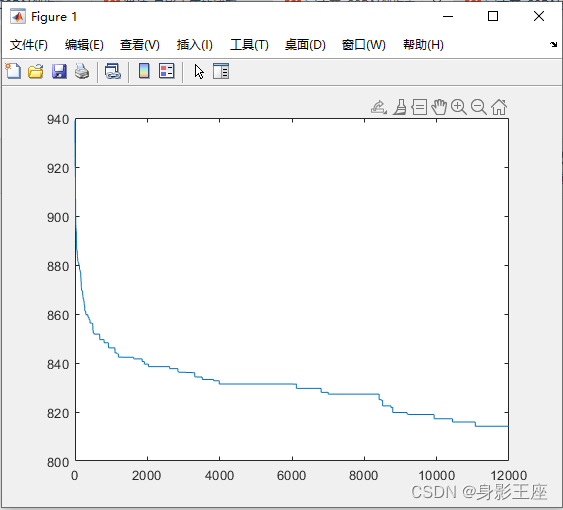
CPSO_Hk( Repeat the experiment 100 Time , Average. ): The evaluation times are about half less than the above two .
clc;clear;clearvars;
%  Random generation 20 Data ,P10 individual ,Q10 individual
num_initial1 = 10;
num_initial2 = 10;
num_vari = 60;
%  Search range
upper_bound = 5.12;
lower_bound = -5.12;
%  Calculate during iteration y Total number of values
eval_num = 12000;
% K Represents the number of partitioned subspaces ,sub_num Represents the dimension of each subspace
K = 6;
sub_num = num_vari / K;
%  The number of iterations of the algorithm
iter = eval_num / K;
w = 1;
%  Random generation 10\10 Data , And obtain its evaluation value
sample_x1 = lhsdesign(num_initial1, num_vari).*(upper_bound - lower_bound) + lower_bound.*ones(num_initial1, num_vari);
sample_y1 = Rastrigin(sample_x1);
sample_x2 = lhsdesign(num_initial2, num_vari).*(upper_bound - lower_bound) + lower_bound.*ones(num_initial2, num_vari);
sample_y2 = Rastrigin(sample_x2);
Fmin = zeros(iter, 1);
aver_Fmin = zeros(iter, 1);

for n = 1 : 100
    n1 = 1;
    %  Initialize some parameters
    pbestx1 = sample_x1;
    pbesty1 = sample_y1;
    pbestxx = sample_x2;
    pbestyy = sample_y2;
    %  Current location information presentx
    presentx1 = lhsdesign(num_initial1, num_vari).*(upper_bound - lower_bound) + lower_bound.*ones(num_initial1, num_vari);
    presentxx = lhsdesign(num_initial2, num_vari).*(upper_bound - lower_bound) + lower_bound.*ones(num_initial2, num_vari);
    vx1 = sample_x1;
    vxx = sample_x2;
    [fmin1, gbest1] = min(pbesty1);
    [fmin2, gbest2] = min(pbestyy);
    global_best_x1 = pbestx1(gbest1, :);
    fprintf("n: %.4f\n", n);
    % fprintf("iter 0 fmin: %.4f\n", fmin);
    for i = 1 : iter
        for i1 = 1 : K
            ind = ((1 + (i1 - 1) * sub_num) : i1 * sub_num);
            r1 = rand(num_initial1, sub_num);
            % cpso Update the location of the next step , Here you can set the boundary if it exceeds the search range
            vx1(:, ind) = w.*vx1(:, ind) + 2 * r1 .* (pbestx1(:, ind) - presentx1(:, ind)) + 2 * r1 .* (pbestx1(gbest1, ind) - presentx1(:, ind));
            vx2 = vx1(:, ind);
            vx2(vx2 > upper_bound) = upper_bound;
            vx2(vx2 < lower_bound) = lower_bound;
            vx1(:, ind) = vx2;
            presentx1(:, ind) = presentx1(:, ind) + vx2;
            presentx2 = presentx1(:, ind);
            presentx2(presentx2 > upper_bound) = upper_bound;
            presentx2(presentx2 < lower_bound) = lower_bound;
            presentx1(:, ind) = presentx2;

            presentx3 = repmat(global_best_x1, num_initial1, 1);
            presentx3(:, ind) = presentx2;
            presenty1 = Rastrigin(presentx3);

            %  Update the best location for each individual
            pbestx2 = pbestx1(:, ind);
            pbestx2(presenty1 < pbesty1, :) = presentx2(presenty1 < pbesty1, :);
            pbestx1(:, ind) = pbestx2;
            pbesty1(presenty1 < pbesty1, :) = presenty1(presenty1 < pbesty1, :);

            %  Update the best location of all individuals
            [fmin1, gbest1] = min(pbesty1);
            global_best_x1 = pbestx1(gbest1, :);
        end

        %  In this paper, the s/2 Namely num_initial2, The following is PSO Algorithm
        ki = randi(num_initial2);
        while ki == gbest2
            ki = randi(num_initial2);
        end
        %  Information exchange
        presentxx(ki, :) = global_best_x1;
        r2 = rand(num_initial2, num_vari);
        % pso Update the location of the next step , Here you can set the boundary if it exceeds the search range
        vxx = w.*vxx + 2 * r2 .* (pbestxx - presentxx) + 2 * r2 .* (pbestxx(gbest2, :) - presentxx);
        vxx(vxx > upper_bound) = upper_bound;
        vxx(vxx < lower_bound) = lower_bound;
        presentxx = presentxx + vxx;
        presentxx(presentxx > upper_bound) = upper_bound;
        presentxx(presentxx < lower_bound) = lower_bound;
        presentyy = Rastrigin(presentxx);
        %  Update the best location for each individual
        pbestxx(presentyy < pbestyy, :) = presentxx(presentyy < pbestyy, :);
        pbestyy(presentyy < pbestyy, :) = presentyy(presentyy < pbestyy, :);
        %  Update the best location of all individuals
        [fmin2, gbest2] = min(pbestyy);
        %  Information exchange
        for i2 = 1 : K
            kj = randi(num_initial1);
            while kj == gbest1
                kj = randi(num_initial1);
            end
            ind2 = ((1 + (i2 - 1) * sub_num) : i2 * sub_num);
            presentx1(kj, ind2) = pbestxx(gbest2, ind2);
        end

        % Get the global optimal value
        if(fmin2 > fmin1)
            fmin = fmin1;
        else
            fmin = fmin2;
        end
        Fmin(n1, 1) = fmin;
        n1 = n1 +1;
        %fprintf("iter %d fmin: %.4f\n", i, fmin);
    end
    aver_Fmin = aver_Fmin + Fmin;
end
aver_Fmin = aver_Fmin ./ 100;
plot(aver_Fmin);
although CPSO_Sk and CPSO_Hk Compared with PSO Not much improvement , But its idea of delimiting molecular space is still very rare . In fact, with the improvement of the problem dimension ,CPSO_Sk and CPSO_Hk The running time of is less than PSO Of , Because the total operation is reduced . And from the end result CPSO_Hk Performance of >CPSO_Sk>PSO.
边栏推荐
- How does Huawei enable debug and how to make an image port
- Four commonly used techniques for anti aliasing
- Leetcode 208. Implement trie (prefix tree)
- 1791. Find the central node of the star diagram / 1790 Can two strings be equal by performing string exchange only once
- Leetcode daily question solution: 1189 Maximum number of "balloons"
- PHP error what is an error?
- Basic process and testing idea of interface automation
- leetcode刷题_验证回文字符串 Ⅱ
- Five challenges of ads-npu chip architecture design
- [day 30] given an integer n, find the sum of its factors
猜你喜欢
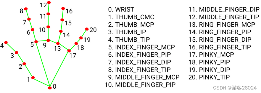
3D视觉——4.手势识别(Gesture Recognition)入门——使用MediaPipe含单帧(Singel Frame)和实时视频(Real-Time Video)
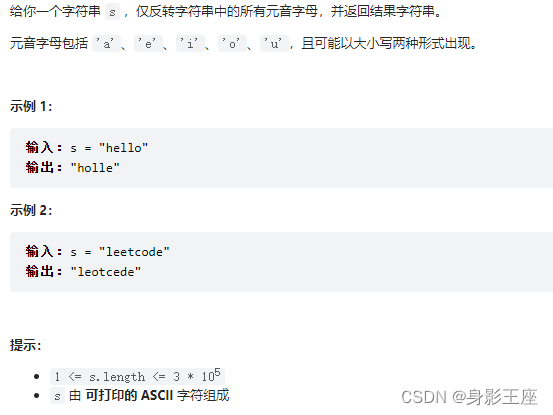
leetcode刷题_反转字符串中的元音字母
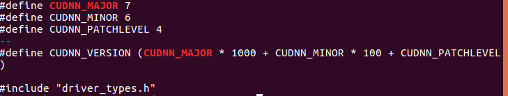
Ubantu check cudnn and CUDA versions
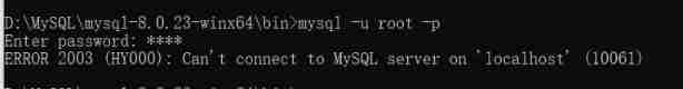
About error 2003 (HY000): can't connect to MySQL server on 'localhost' (10061)
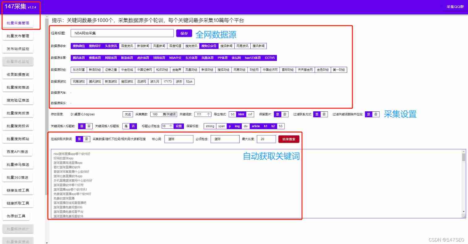
Xunrui CMS plug-in automatically collects fake original free plug-ins

What is the most suitable book for programmers to engage in open source?

How to see the K-line chart of gold price trend?

Ordinary people end up in Global trade, and a new round of structural opportunities emerge

282. Stone consolidation (interval DP)

XSS learning XSS lab problem solution
随机推荐
Spir - V premier aperçu
Recursive method converts ordered array into binary search tree
[Yu Yue education] Liaoning Vocational College of Architecture Web server application development reference
Basic process and testing idea of interface automation
The inconsistency between the versions of dynamic library and static library will lead to bugs
FFT learning notes (I think it is detailed)
[技术发展-28]:信息通信网大全、新的技术形态、信息通信行业高质量发展概览
关于softmax函数的见解
什么是弱引用?es6中有哪些弱引用数据类型?js中的弱引用是什么?
How does Huawei enable debug and how to make an image port
After 95, the CV engineer posted the payroll and made up this. It's really fragrant
Superfluid_ HQ hacked analysis
BiShe - College Student Association Management System Based on SSM
Condition and AQS principle
[day 30] given an integer n, find the sum of its factors
Format code_ What does formatting code mean
Docker compose configures MySQL and realizes remote connection
CocoaPods could not find compatible versions for pod 'Firebase/CoreOnly'
Four commonly used techniques for anti aliasing
Finding the nearest common ancestor of binary tree by recursion