当前位置:网站首页>Skimage learning (1)
Skimage learning (1)
2022-07-07 17:02:00 【Original knowledge】
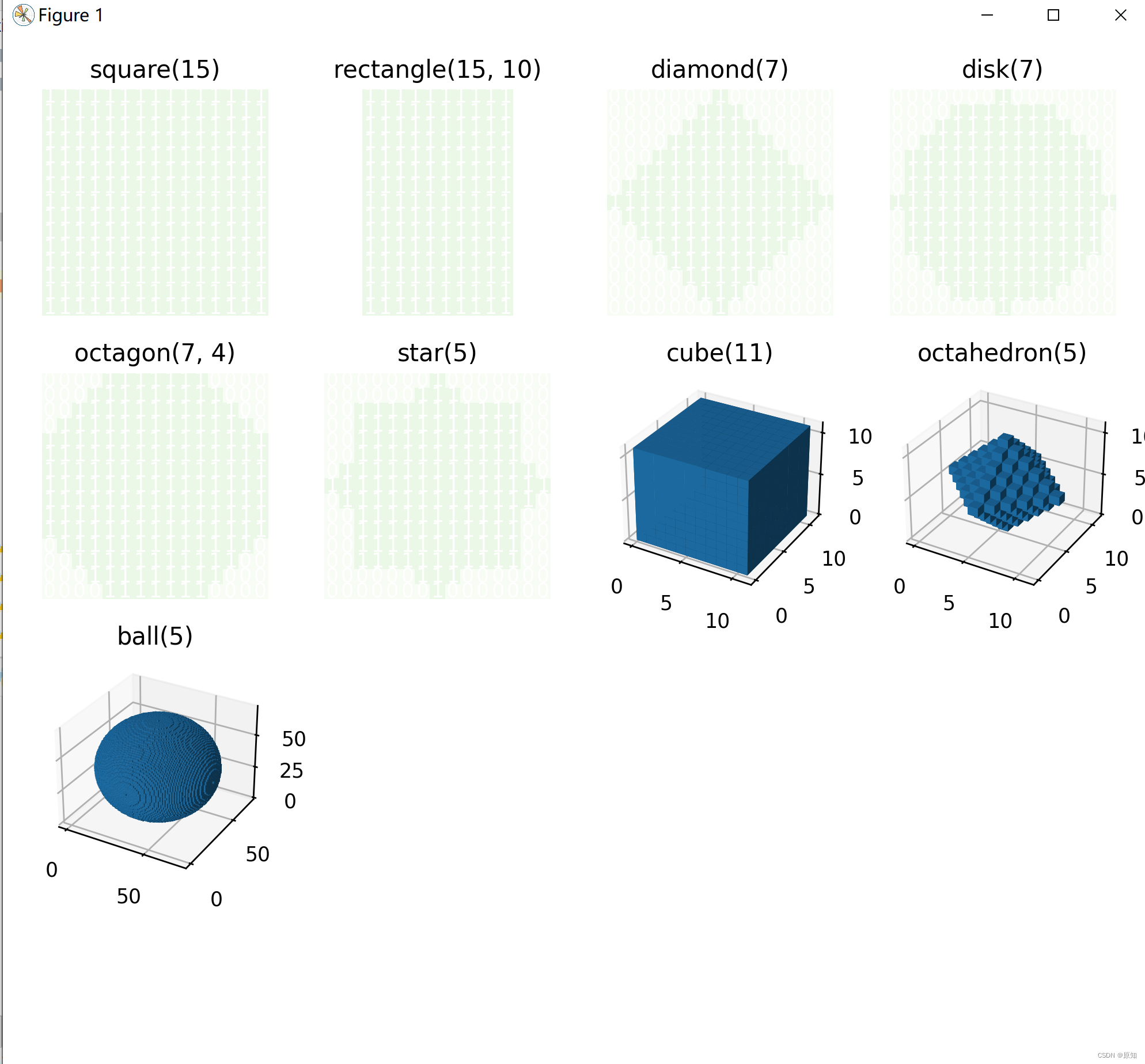
1、 Generate structured elements
This example shows how to use skimage The function in . Generate morphology of structural elements . The title of each graph represents the function call .
import numpy as np
import matplotlib.pyplot as plt
from mpl_toolkits.mplot3d import Axes3D

from skimage.morphology import (square, rectangle, diamond, disk, cube,
                                octahedron, ball, octagon, star)
# Square 、 Rectangle 、 The diamond 、 The disk 、 Cube 、 Octahedron 、 sphere 、 Octagon 、 Stars
# Generate 2D and 3D structuring elements.
struc_2d = {

    "square(15)": square(15),
    "rectangle(15, 10)": rectangle(15, 10),
    "diamond(7)": diamond(7),
    "disk(7)": disk(7),
    "octagon(7, 4)": octagon(7, 4),
    "star(5)": star(5)
}

struc_3d = {

    "cube(11)": cube(11),
    "octahedron(5)": octahedron(5),
    "ball(5)": ball(35),
"ball(5)": ball(35),
}

# Visualize the elements.
fig = plt.figure(figsize=(8, 8))

idx = 1
#tems() Function returns a list of traversable ( Key value ) Tuple array .
''' plt.text(x, y, string, weight="bold", color="b") x:  Abscissa of the location of the content of the note text  y: The ordinate of the location where the annotation text content is located  string: Note text content ,struc[i, j] number 0、1 weight: Thickness style of annotation text content  '''
for title, struc in struc_2d.items():
    ax = fig.add_subplot(4, 4, idx)#3 That's ok 3 Column , The position is
    ax.imshow(struc, cmap="Greens", vmin=0, vmax=12)#ax Parameters are used to limit the range of values , Only will vmin and vmax Mapping values between , Usage is as follows
    for i in range(struc.shape[0]):
        for j in range(struc.shape[1]):
            ax.text(j, i, struc[i, j], ha="center", va="center", color="w")
    ax.set_axis_off()
    ax.set_title(title)
    idx += 1

for title, struc in struc_3d.items():
    ax = fig.add_subplot(4, 4, idx, projection=Axes3D.name)
    ax.voxels(struc)
    ax.set_title(title)
    idx += 1

fig.tight_layout()
plt.show()
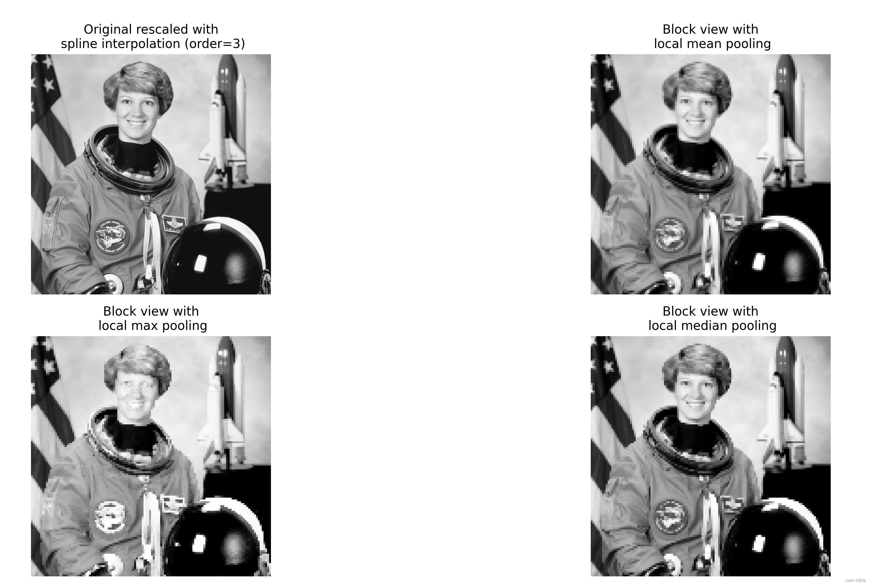
2、 Images / Block view on array
This example demonstrates skimage.util() Medium view_as_blocks Use . When one wants to perform local operations on non overlapping image blocks , Block views are very useful . We use it skimage Medium astronaut. data , And its “ segmentation ” For all aspects . then , On each block , We can either gather the average value of this block , Maximum or median . The results are displayed together , Zoom the original astronaut image together with a third-order spline interpolation .
import numpy as np
from scipy import ndimage as ndi
from matplotlib import pyplot as plt
import matplotlib.cm as cm

from skimage import data
from skimage import color
from skimage.util import view_as_blocks


# get astronaut from skimage.data in grayscale
l = color.rgb2gray(data.astronaut())
#img=skimage.io.imread('11.jpg',)
#l = color.rgb2gray(img)
# size of blocks
block_shape = (4,4)

# Divide the astronaut picture into matrix blocks ( The size is block_shape)
view = view_as_blocks(l, block_shape)

#  The last two dimensions merge into one , Become an array for easy operation
#img.shape[0]: The vertical size of the image ( Height ) img.shape[1]: The horizontal size of the image ( Width )
flatten_view = view.reshape(view.shape[0], view.shape[1], -1)

#  By taking the “ mean value ”、“ Maximum ” or “ The median ” Resample the image .mean() The functionality : Find the mean
mean_view = np.mean(flatten_view, axis=2)
max_view = np.max(flatten_view, axis=2)
median_view = np.median(flatten_view, axis=2)

#  Draw a subgraph ,sharex and sharey: surface ⽰ Whether the attributes of the coordinate axis are the same
fig, axes = plt.subplots(2, 2, figsize=(8, 8), sharex=True, sharey=True)
ax = axes.ravel()# Flatten the multidimensional data to ⼀ D data , It is equivalent to  reshape(-1, order=order) .

''' https://vimsky.com/examples/usage/python-scipy.ndimage.zoom.html https://www.jianshu.com/p/909851f46411 ndi.zoom(input,zoom,output=None,order,mode='constant',cval=0.0,prefilter=True) Scale the array . Scale the array using spline interpolation in the requested order . input:  Input pictures as an array  zoom: Floating point numbers or arrays . If it's a floating point number , Zoom in and out the same multiple for each axis . If it's an array , Then assign a value to each axis . output: Output , The default is None order: integer ( Range 0-5) The order of spline interpolation , The default is 3. See later  '''
l_resized = ndi.zoom(l, 2, order=3)
ax[0].set_title("Original rescaled with\n spline interpolation (order=3)")
ax[0].imshow(l_resized, extent=(-0.5, 128.5, 128.5, -0.5),
             cmap=cm.Greys_r)

ax[1].set_title("Block view with\n local mean pooling")
ax[1].imshow(mean_view, cmap=cm.Greys_r)

ax[2].set_title("Block view with\n local max pooling")
ax[2].imshow(max_view, cmap=cm.Greys_r)

ax[3].set_title("Block view with\n local median pooling")
ax[3].imshow(median_view, cmap=cm.Greys_r)

for a in ax:
    a.set_axis_off()

fig.tight_layout()
plt.show()
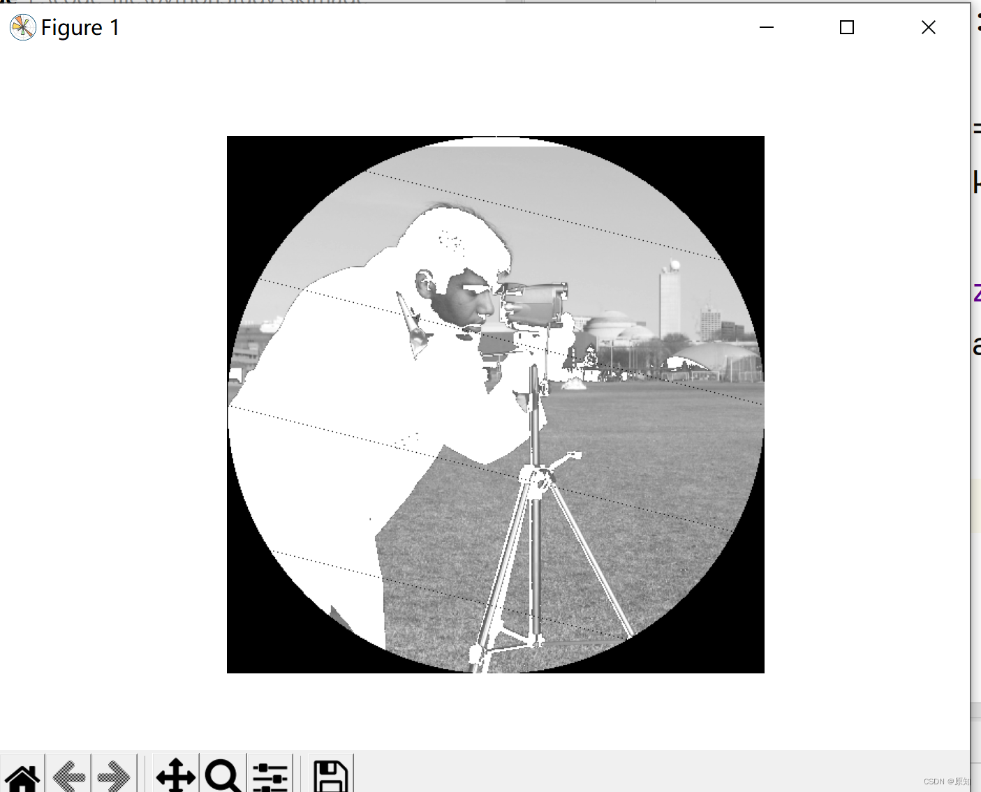
3、 Easy to use NumPy Operation to process images
This script explains how to use the basic NumPy operation , For example, slice 、 Shielding and fancy indexing , To modify the pixel value of the image .
# Use basic  NumPy  operation , For example, slice 、 Shielding and fancy indexing , To modify the pixel value of the image .
import numpy as np
from skimage import data
import matplotlib.pyplot as plt

# Read in ,camera yes ndarray Array of
camera = data.camera()
camera[:10] = 0# The first 0-9 Set as 0
mask = camera < 87#‘< ’ For conditional statements , Only return “ True and false ”. take camera Medium pixel value <87 The position of is marked as true, Others are false
camera[mask] = 255# recycling mask Marked position (true and false), Will be worth true The value of the set 255
inds_x = np.arange(len(camera))# Abscissa 0-511,arange(a,b,c) Function generation a~b( barring b), The interval is c An array of , ginseng 511 End point , Starting point 0, Step size is the default value 1.
inds_y = (4 * inds_x) % len(camera)# The generation step is 4 Array of , Ordinate
camera[inds_x, inds_y] = 0 # Press inds_x, inds_y The value of sets the pixel to zero
l_x, l_y = camera.shape[0], camera.shape[1]# Read the matrix length
print(l_x,l_y)
X, Y = np.ogrid[:l_x, :l_y]# Produce two long 512 Two dimensional array of
print(X,Y)
outer_disk_mask = (X - l_x / 2)**2 + (Y - l_y / 2)**2 > (l_x / 2)**2# Generate circular grid coordinates
camera[outer_disk_mask] = 0 #  Assign , Everything except circles turns black

plt.figure(figsize=(4, 4)) #  establish figure The size ratio of
plt.imshow(camera, cmap='gray') #  Display images
plt.axis('off')
plt.show()
边栏推荐
猜你喜欢
Personal notes of graphics (2)
最新Android面试合集,android视频提取音频
Advanced C language -- function pointer
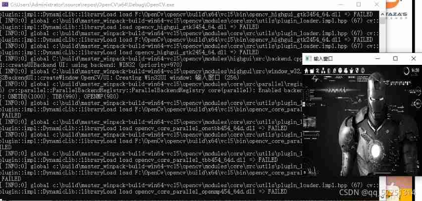
Opencv personal notes
网关Gateway的介绍与使用
The process of creating custom controls in QT to encapsulating them into toolbars (II): encapsulating custom controls into toolbars
运算符
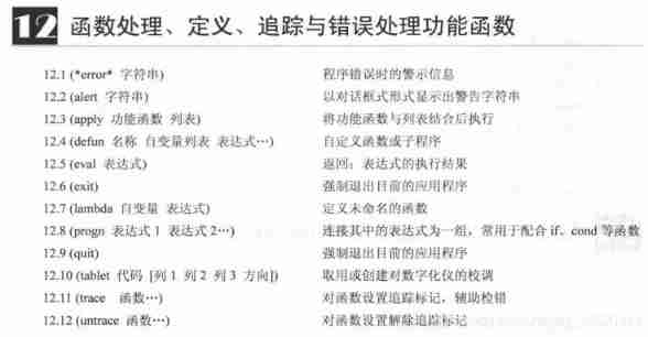
AutoLISP series (3): function function 3
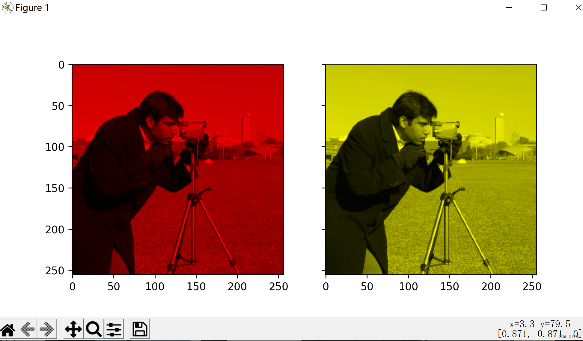
skimage学习(3)——Gamma 和 log对比度调整、直方图均衡、为灰度图像着色
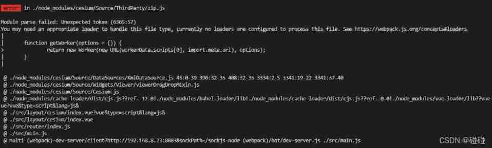
Cesium(3):ThirdParty/zip. js
随机推荐
Prediction - Grey Prediction
正在准备面试,分享面经
谎牛计数(春季每日一题 53)
打造All-in-One应用开发平台,轻流树立无代码行业标杆
Personal notes of graphics (3)
全网“追杀”钟薛高
AutoLISP series (3): function function 3
最新2022年Android大厂面试经验,安卓View+Handler+Binder
Lowcode: four ways to help transportation companies enhance supply chain management
掌握这个提升路径,面试资料分享
LeetCode 1186. Delete once to get the sub array maximum and daily question
Three. JS series (1): API structure diagram-1
字节跳动Android面试,知识点总结+面试题解析
【医学分割】attention-unet
SlashData开发者工具榜首等你而定!!!
skimage学习(3)——Gamma 和 log对比度调整、直方图均衡、为灰度图像着色
LeetCode 1031. Maximum sum of two non overlapping subarrays
面向接口编程
ByteDance Android gold, silver and four analysis, Android interview question app
Master this promotion path and share interview materials