当前位置:网站首页>[statistical learning method] learning notes - support vector machine (I)
[statistical learning method] learning notes - support vector machine (I)
2022-07-07 12:34:00 【Sickle leek】
Statistical learning methods learning notes —— Support vector machine ( On )
Support vector machine (support vector machines, SVM) yes A two class classification model . Its basic model is Define the linear classifier with the largest interval in the feature space , The maximum spacing makes it different from the perceptron ; Support vector machines also include Nuclear skills , This makes it essentially Nonlinear classifier . The learning strategy of support vector machine is Maximize spacing , It can be formalized as a solution Convex quadratic programming (convex quadratic programming) The problem of , It's also equivalent to regularized Minimization of hinge loss function . The learning algorithm of support vector machine is an optimization algorithm for solving convex quadratic programming .
Support vector machine learning methods include building models from simple to complex :
- Linearly separable SVM: When the training data is linearly separable , adopt
Maximize hard spacing, Learn a linear classifier , Linear separable SVM, also called Hard spacing SVM. - linear SVM: When the training data is approximately linearly separable , adopt
Maximize soft spacing, Also learn a linear classifier , Linear SVM, also called Soft space SVM. - nonlinear SVM: When the training data is linear and indivisible , By using
Nuclear skillsAndMaximize soft spacing, Study nonlinear SVM.
Kernel function It means mapping the input from the input space to the feature space to get the inner product between the feature vectors . Nonlinearity can be learned by using kernel functions SVM, It is equivalent to learning linearity implicitly in high-dimensional feature space SVM. The method is called Nuclear method , The nuclear method is better than SVM More general machine learning methods .
1. Linear separable support vector machine and hard interval maximization
1.1 Linear separable support vector machine
Suppose the input space is Euclidean space or discrete set , The feature space is Euclidean space or Hilbert space . Linear separable support vector machine 、 Linear support vector machine assumes that the elements of the two spaces correspond one to one , The input in the input space is mapped to the feature vector in the feature space .
Nonlinear support vector machine uses a nonlinear mapping from input space to feature space to map input into feature vector . therefore , Input is transformed from input space to feature space , The learning of support vector machine is carried out in feature space .
Suppose a training data set on the feature space is given T = { ( x 1 , y 1 ) , ( x 2 , y 2 ) , . . . , ( x N , y N ) } T=\{(x_1, y_1), (x_2, y_2), ..., (x_N, y_N)\} T={ (x1,y1),(x2,y2),...,(xN,yN)}, among x i ∈ X = R n x_i\in \mathcal{X}=R^n xi∈X=Rn, y i ∈ y = { + 1 , − 1 } , i = 1 , 2 , . . . , N y_i\in \mathcal{y}=\{+1, -1\}, i=1,2,..., N yi∈y={ +1,−1},i=1,2,...,N. x i x_i xi For the first time i i i eigenvectors , It also becomes an example . y i y_i yi by x i x_i xi Class tags for . When y i = + 1 y_i=+1 yi=+1 when , call x i x_i xi For example ; When y i = − 1 y_i=-1 yi=−1 when , call x i x_i xi The negative example is . ( x i , y i ) (x_i, y_i) (xi,yi) Is the sample point . Suppose that the training data set is linearly separable .
The goal of learning is to find a separated hyperplane in the feature space , Can divide instances into different classes . The separation hyperplane corresponds to the equation w ⋅ x + b = 0 w\cdot x + b=0 w⋅x+b=0, It consists of the normal vector w w w And intercept b b b decision , You can use ( w , b ) (w,b) (w,b) To express . The separation hyperplane divides the feature space into two parts , Some are positive classes , Some are negative classes . The normal vector points to a positive class on one side , The other side is negative .
In a general way , When the training data set is linearly separable , There are infinite separating hyperplanes that can correctly classify the two types of data . The perceptron uses the strategy of minimizing misclassification , Find the separating hyperplane , But there are infinite solutions . And linear separable support vector machine is to find the largest separation hyperplane , This is the only .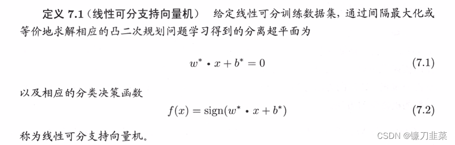
1.2 Function interval and geometric interval
Generally speaking , The distance between a point and the separation hyperplane can indicate the degree of certainty of classification prediction . In the hyperplane w ⋅ x + b = 0 w\cdot x + b =0 w⋅x+b=0 In certain cases , ∣ w ⋅ x + b ∣ |w\cdot x +b| ∣w⋅x+b∣ To be able to represent a point relatively x x x The distance from the hyperplane , and w ⋅ x + b w\cdot x +b w⋅x+b Symbol with class notation y y y Whether the symbols of are consistent can indicate whether the classification is correct . So it can be used y ( w ⋅ x + b ) y(w\cdot x +b) y(w⋅x+b) To show the correctness and certainty of classification . This is it. The function between (functional margin) The concept of .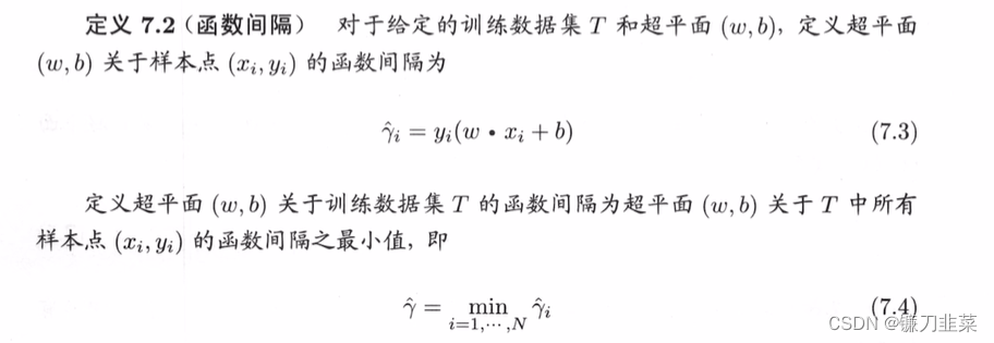
The function interval can express the accuracy and certainty of classification prediction . But if it changes proportionally w w w and b b b, The hyperplane hasn't changed , But the function interval becomes the original 2 times .
To ensure uniqueness , You can separate hyperplane normal vectors w w w Put some restrictions on , Such as standardization , ∣ ∣ w ∣ ∣ = 1 ||w||=1 ∣∣w∣∣=1, This makes the interval definite . At this time, the function interval becomes the geometric interval (geometric margin).
In a general way , When the sample point ( x i , y i ) (x_i, y_i) (xi,yi) Hyperplane ( w , b ) (w, b) (w,b) When correctly classified , spot x i x_i xi And hyperplane ( w , b ) (w, b) (w,b) The distance is
γ i = y i ( w ∣ ∣ w ∣ ∣ ⋅ x i + b ∣ ∣ w ∣ ∣ ) \gamma_i=y_i(\frac{w}{||w||} \cdot x_i + \frac{b}{||w||}) γi=yi(∣∣w∣∣w⋅xi+∣∣w∣∣b)
From this fact, the concept of geometric interval is derived .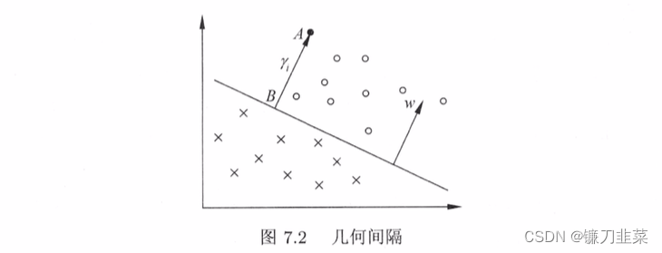
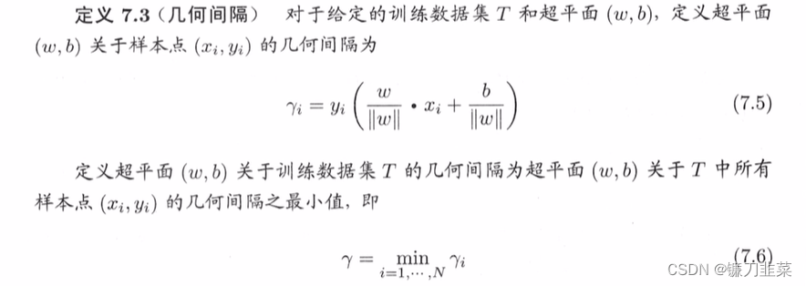
From the definition of function interval and geometric interval , There is the following relationship between function interval and geometric interval : γ i = γ ^ i ∣ ∣ w ∣ ∣ \gamma_i=\frac{\hat{\gamma}_i}{||w||} γi=∣∣w∣∣γ^i γ = γ ^ ∣ ∣ w ∣ ∣ \gamma = \frac{\hat{\gamma}}{||w||} γ=∣∣w∣∣γ^ If ∣ ∣ w ∣ ∣ = 1 ||w||=1 ∣∣w∣∣=1, Then the function interval is equal to the geometric interval . If the hyperplane parameter w w w and b b b Change in proportion ( The hyperplane does not change ), The function interval also changes in this proportion , And the geometric spacing remains the same .
1.3 Maximize spacing
The basic idea of support vector machine learning is to solve the separation hyperplane which can correctly divide the training data set and has the largest geometric interval . For linearly separable training sets , There are infinite number of linearly separable hyperplanes ( Equivalent to perceptron ), But the separated hyperplane with the largest geometric spacing is the only one . The maximum spacing here is also known as Maximize hard spacing ( Corresponding to the maximization of soft interval when the training data set to be discussed is approximately linearly separable ).
Maximize spacing : Finding the hyperplane with the largest geometric interval means classifying the training data with sufficient confidence . That is to say, not only the positive and negative instance points are separated , And for hard to distinguish examples ( The closest point to the hyperplane ) There is also enough certainty to separate them .
- Maximum separation hyperplane
Next, consider how to find a separation hyperplane with the largest geometric spacing , That is, the maximum separation hyperplane . In particular , This problem can be expressed as the following constrained optimization problem
max w , b γ \max_{w,b} \gamma w,bmaxγ s . t . y i ( w ∣ ∣ w ∣ ∣ ⋅ x i + b ∣ ∣ w ∣ ∣ ) ≥ γ , i = 1 , 2 , . . . , N s.t. \ y_i(\frac{w}{||w||}\cdot x_i+\frac{b}{||w||})\ge \gamma, i=1,2,...,N s.t. yi(∣∣w∣∣w⋅xi+∣∣w∣∣b)≥γ,i=1,2,...,N
That is, we want to maximize the hyperplane ( w , b ) (w,b) (w,b) On the geometric interval of the training data set γ \gamma γ, The constraint represents a hyperplane ( w , b ) (w,b) (w,b) The geometric interval of each training sample point is at least γ \gamma γ.
Consider the relationship between geometric interval and functional interval γ = γ ^ ∣ ∣ w ∣ ∣ \gamma = \frac{\hat{\gamma}}{||w||} γ=∣∣w∣∣γ^, The question can be rewritten as
max w , b γ ^ ∣ ∣ w ∣ ∣ \max_{w,b} \frac{\hat{\gamma}}{||w||} w,bmax∣∣w∣∣γ^ s . t . y i ( w ⋅ x i + b ) ≥ γ ^ , i = 1 , 2 , . . . , N s.t. y_i(w\cdot x_i+b)\ge \hat{\gamma}, i=1,2,...,N s.t.yi(w⋅xi+b)≥γ^,i=1,2,...,N
The function between γ \gamma γ The value of does not affect the solution of the optimization problem . Assume that w w w and b b b Change proportionally to λ w \lambda w λw and KaTeX parse error: Undefined control sequence: \lambdab at position 1: \̲l̲a̲m̲b̲d̲a̲b̲, At this time, the function interval is called λ γ ^ \lambda \hat{\gamma} λγ^, This change of function interval has no effect on the inequality constraint of the above optimization problem , It also has no effect on the optimization of the objective function . such , You can take γ ^ = 1 \hat{\gamma} = 1 γ^=1.
Also note the maximization 1 ∣ ∣ w ∣ ∣ \frac{1}{||w||} ∣∣w∣∣1 And minimize 1 2 ∣ ∣ w ∣ ∣ 2 \frac{1}{2}||w||^2 21∣∣w∣∣2 It is equivalent. , So we get the following optimization problem
min w , b 1 2 ∣ ∣ w ∣ ∣ 2 \min_{w,b} \frac{1}{2}||w||^2 w,bmin21∣∣w∣∣2 s . t . y i ( w ⋅ x i + b ) − 1 ⩾ 0 , i = 1 , 2 , . . . , N s.t. y_i(w\cdot x_i+b)−1⩾0, i=1,2,...,N s.t.yi(w⋅xi+b)−1⩾0,i=1,2,...,N
This is a convex quadratic programming (convex quadratic programming) problem .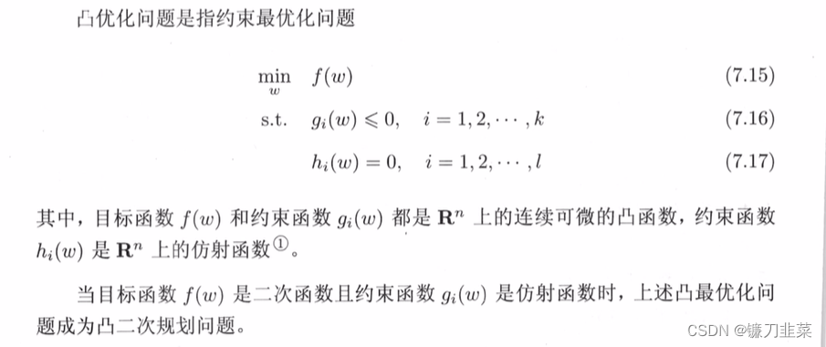
Solving constrained optimization problems , obtain w ∗ w∗ w∗ and b ∗ b∗ b∗, We can get the maximum separation hyperplane w ∗ ⋅ x + b ∗ = 0 w^* \cdot x + b^* = 0 w∗⋅x+b∗=0 And classification decision function f ( x ) = s i g n ( w ∗ ⋅ x + b ∗ ) f(x) = sign(w^* \cdot x + b^*) f(x)=sign(w∗⋅x+b∗), The linear separable support vector machine model .
Algorithm : Linear separable support vector machine learning algorithm —— Maximum interval method
Input : Linearly separable training data set T = { ( x 1 , y 1 ) , ( x 2 , y 2 ) , . . . , ( x N , y N ) } T=\{(x_1, y_1), (x_2, y_2), ..., (x_N, y_N)\} T={ (x1,y1),(x2,y2),...,(xN,yN)}, among x i ∈ X = R n x_i\in \mathcal{X}=R^n xi∈X=Rn, y i ∈ y = { + 1 , − 1 } , i = 1 , 2 , . . . , N y_i\in \mathcal{y}=\{+1, -1\}, i=1,2,..., N yi∈y={ +1,−1},i=1,2,...,N;
Output : Maximum separation hyperplane and classification decision function .
(1) Construct and solve constrained optimization problems : min w , b 1 2 ∣ ∣ w ∣ ∣ 2 \min_{w, b} \ \frac{1}{2}||w||^2 w,bmin 21∣∣w∣∣2 s . t . y i ( w ⋅ x i + b ) − 1 ≥ 0 , i = 1 , 2 , . . . , N s.t. \ y_i(w\cdot x_i + b)-1 \ge 0, i=1,2, ..., N s.t. yi(w⋅xi+b)−1≥0,i=1,2,...,N
Find the optimal solution w ∗ , b ∗ w^*, b^* w∗,b∗
(2) So we get the separation hyperplane : w ∗ ⋅ x + b ∗ = 0 w^* \cdot x + b^* = 0 w∗⋅x+b∗=0 Classification decision function f ( x ) = s i g n ( w ∗ ⋅ x + b ∗ ) f(x)=sign (w^* \cdot x + b^*) f(x)=sign(w∗⋅x+b∗)
Existence and uniqueness of maximal separation hyperplane
The maximal separation hyperplane of linearly separable training data sets exists and is unique .
Theorem ( Existence and uniqueness of maximal separation hyperplane ): If the training data set T Linearly separable , Then the maximum separation hyperplane that can completely and correctly classify the sample points in the training data set exists and is unique .Support vector and interval boundary
In the case of linear separability , The instance of the sample point closest to the separation hyperplane in the sample point of the training data set is called support vector (support vector). Support vector is the point that makes the following equal sign true , namely y i ( w ⋅ x i + b ) − 1 = 0 y_i(w\cdot x_i + b)-1=0 yi(w⋅xi+b)−1=0
Yes y i = + 1 y_i=+1 yi=+1 The normal point of , The support vector is in the hyperplane H 1 : w ⋅ x + b = 1 H_1: w\cdot x + b = 1 H1:w⋅x+b=1 On , Yes y i = − 1 y_i=-1 yi=−1 Negative example point of , The support vector is in the hyperplane H 2 : w ⋅ + b = − 1 H_2: w\cdot +b = -1 H2:w⋅+b=−1 On . Pictured 7.3 Shown , stay H 1 H_1 H1 and H 2 H_2 H2 The point on is the support vector .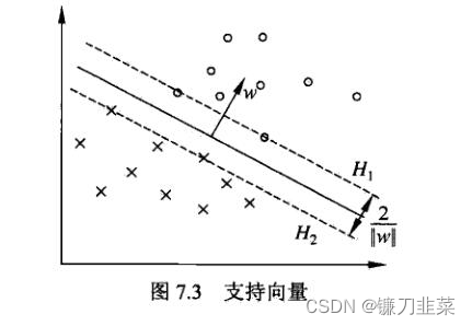
Separation boundary : H 1 H_1 H1 and H 2 H_2 H2 parallel , No instance point falls between them . H 1 H_1 H1 And H 2 H_2 H2 Form a long belt between , The separation hyperplane is parallel to them and located in their center . The width of the length , namely H 1 H_1 H1 and H 2 H_2 H2 The distance between them is called interval , The interval depends on the normal vector separating the hyperplanes w w w, be equal to 2 ∣ ∣ w ∣ ∣ 2||w|| 2∣∣w∣∣, H 1 H_1 H1 and H 2 H_2 H2 be called Separation boundary .
When deciding to separate hyperplanes , Only support vectors work . If we move the support vector, we will change the solution , But if you move other instance points outside the interval boundary , Even get rid of the dots , The solution will not change .
Because support vector plays a decisive role in determining hyperplane , So this method is calledSupport vector machine. The number of support vectors is usually very small , So SVM consists of very few “ important ” Determination of training samples .
1.4 The dual algorithm of learning
Dual algorithm (dual algorithm): In order to solve the optimization problem of linear separable support vector machine , Think of it as a primitive optimization problem , Applying Lagrange duality , By solving duality (dual problem) The problem gets the original problem (primal problem) The best solution . Doing so advantage : One is that dual problems are often easier to solve ; The second is to introduce kernel function naturally , And then extended to the nonlinear classification problem .
First , Construct Lagrange function (Lagrange function). So , For every inequality constraint, Lagrange multipliers are introduced (lagrange multiplier) α i ≥ 0 , i = 1 , 2 , . . . , N \alpha_i \ge 0, i=1,2,...,N αi≥0,i=1,2,...,N, Define the Lagrange function :
L ( w , b , α ) = 1 2 ∣ ∣ w ∣ ∣ 2 − ∑ i = 1 N α i y i ( w ⋅ x i + b ) + ∑ i = 1 N α i L(w, b, \alpha)=\frac{1}{2}||w||^2 - \sum_{i=1}^N \alpha_i y_i(w\cdot x_i + b)+\sum_{i=1}^N \alpha_i L(w,b,α)=21∣∣w∣∣2−i=1∑Nαiyi(w⋅xi+b)+i=1∑Nαi among α = ( α 1 , α 2 , . . . , α N ) T \alpha = (\alpha_1, \alpha_2,...,\alpha_N)^T α=(α1,α2,...,αN)T For the Lagrange multiplier vector .
According to Lagrangian duality , The dual problem of the primal problem makes the minimax problem : max α min w , b L ( w , b , α ) \max_{\alpha}\min_{w,b} L(w, b,\alpha) αmaxw,bminL(w,b,α)
therefore , In order to get the solution of the dual problem , We need to ask first. L ( w , b , α ) L(w, b, \alpha) L(w,b,α) Yes w , b w,b w,b The smallest of , Ask for the right again α \alpha α It's huge .
(1) seek min w , b L ( w , b , α ) \min_{w,b} L(w,b,\alpha) minw,bL(w,b,α)
Let's take the Lagrange function L ( w , b , α ) L(w,b,\alpha) L(w,b,α) Respectively for w , b w,b w,b Take the partial derivative and make it equal to 0.
have to : w = ∑ i = 1 N α i y i x i w = \sum_{i=1}^N \alpha_i y_i x_i w=i=1∑Nαiyixi ∑ i = 1 N α i y i = 0 \sum_{i=1}^N \alpha_i y_i =0 i=1∑Nαiyi=0
Bring it into Lagrange function , Immediate :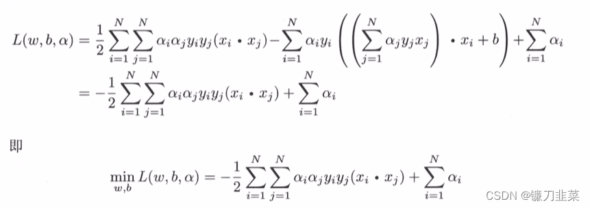
(2) seek min w , b L ( w , b , α ) \min_{w,b} L(w,b, \alpha) minw,bL(w,b,α) Yes α \alpha α It's huge , That is, the dual problem .
Convert the objective function of the above formula from seeking maximum to seeking minimum , The following equivalent dual optimization problem is obtained :
adopt KKT The conditional solution of the dual problem can be obtained :
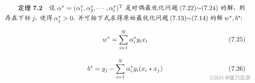
w ∗ = ∑ i = 1 N α i ∗ y i ∗ x i ∗ w^* = \sum_{i=1}^N \alpha_i^*y_i^*x_i^* w∗=i=1∑Nαi∗yi∗xi∗ b ∗ = y j − ∑ i = 1 N α i ∗ y i ( x i ⋅ x j ) b^*=y_j-\sum_{i=1}^N\alpha_i^*y_i(x_i\cdot x_j) b∗=yj−i=1∑Nαi∗yi(xi⋅xj)
According to this theorem , Can be written as a hyperplane ∑ i = 1 N α i ∗ y i ( x ⋅ x i ) + b ∗ = 0 \sum_{i=1}^N \alpha_i^* y_i(x\cdot x_i)+b^*=0 i=1∑Nαi∗yi(x⋅xi)+b∗=0
The classification decision function can be written as f ( x ) = s i g n { ∑ i = 1 N α i ∗ y i ( x ⋅ x i ) + b ∗ } f(x)=sign\{\sum_{i=1}^N \alpha_i^* y_i(x\cdot x_i)+b^*\} f(x)=sign{ i=1∑Nαi∗yi(x⋅xi)+b∗}
That is to say , The classification decision function depends only on the input x And the inner product of training sample input . The above formula is called the dual form of linear separable support vector machine .
Algorithm : Linear separable support vector machine learning algorithm
Input : Linearly separable training data set T = ( x 1 , y 1 ) , ( x 2 , y 2 ) , . . . , ( x N , y N ) T={(x_1,y_1),(x_2,y_2),...,(x_N,y_N)} T=(x1,y1),(x2,y2),...,(xN,yN), among , x i ∈ X = R n , y i ∈ Y = { − 1 , + 1 } , i = 1 , 2 , . . . , N x_i\in \mathcal{X}=R^n,y_i \in \mathcal{Y}=\{−1,+1\},i=1,2,...,N xi∈X=Rn,yi∈Y={ −1,+1},i=1,2,...,N;
Output : Maximum separation hyperplane and classification decision function .
(1) Construct and solve constrained optimization problems :
min α 1 2 ∑ i = 1 N ∑ j = 1 N α i α j y i y j ( x i ⋅ x j ) − ∑ i = 1 N α i \min_α \frac{1}{2}\sum_{i=1}^N\sum_{j=1}^N \alpha_i\alpha_jy_iy_j(x_i\cdot x_j)−\sum_{i=1}^N \alpha_i αmin21i=1∑Nj=1∑Nαiαjyiyj(xi⋅xj)−i=1∑Nαi s . t . ∑ i = 1 N α i y i = 0 , α i ≥ 0 , i = 1 , 2 , . . . , N s.t.\ \sum_{i=1}^N \alpha_iy_i=0, \ \alpha_i\ge 0,i=1,2,...,N s.t. i=1∑Nαiyi=0, αi≥0,i=1,2,...,N
Find the optimal solution α ∗ = ( α 1 ∗ , α 2 ∗ , . . . , α N ∗ ) T \alpha^∗=(\alpha_1^*,\alpha_2^*,...,\alpha_N^*)^T α∗=(α1∗,α2∗,...,αN∗)T;
(2) Calculation :
w ∗ = ∑ i = 1 N α i ∗ y i x i w^∗=\sum_{i=1}^N \alpha_i^* y_ix_i w∗=i=1∑Nαi∗yixi
And select α ∗ \alpha^∗ α∗ A positive component of α j ∗ > 0 \alpha_j^*>0 αj∗>0, Calculation :
b ∗ = y j − ∑ i = 1 N α i ∗ y i ( x i ⋅ x j ) b^∗=y_j−\sum_{i=1}^N\alpha_i^*y_i(x_i\cdot x_j) b∗=yj−i=1∑Nαi∗yi(xi⋅xj)
(3) Find the separating hyperplane :
w ∗ ⋅ x + b ∗ = 0 w^* \cdot x +b^* = 0 w∗⋅x+b∗=0
Classification decision function :
f ( x ) = s i g n { w ∗ ⋅ x + b ∗ } f(x)=sign\{w^* \cdot x + b^*\} f(x)=sign{ w∗⋅x+b∗}
Definition : Support vector : Consider the primal optimization problem and the dual optimization problem , The training data set corresponds to α i ∗ > 0 \alpha_i^* >0 αi∗>0 Sample point of ( x i , y i ) (x_i, y_i) (xi,yi) Example x i ∈ R n x_i \in R^n xi∈Rn be called Support vector .
2. Linear support vector machine and soft interval maximization
2.1 Linear support vector machines
Support vector machine learning method for linear separable problems , It is not applicable to linear nonseparable training set data , Because at this time, the inequality constraints in the above methods cannot be established . How can we extend it to linear indivisible problems ? This requires modifying the hard interval to maximize , Make it a Maximize soft spacing .
Suppose a training data set on the feature space is given T = { ( x 1 , y 1 ) , ( x 2 , y 2 ) , . . . , ( x N , y N ) } T=\{(x_1, y_1), (x_2, y_2), ..., (x_N, y_N)\} T={ (x1,y1),(x2,y2),...,(xN,yN)}, among x i ∈ X = R n x_i\in \mathcal{X}=R^n xi∈X=Rn, y i ∈ y = { + 1 , − 1 } , i = 1 , 2 , . . . , N y_i\in \mathcal{y}=\{+1, -1\}, i=1,2,..., N yi∈y={ +1,−1},i=1,2,...,N. x i x_i xi For the first time i i i eigenvectors , It also becomes an example . y i y_i yi by x i x_i xi Class tags for . Usually it's , There are some special points in the training data (outlier). After removing these specific points , The set composed of most of the remaining sample points is linearly separable .
Linear indivisibility means that some sample points ( x i , y i ) (x_i,y_i) (xi,yi) Cannot satisfy function interval greater than or equal to 1 Constraints of (7.14). To solve this problem , Sure For each sample point ( x i , y i ) (x_i,y_i) (xi,yi) Introduce a relaxation variable ξ i ⩾ 0 ξ_i⩾0 ξi⩾0, Make the function interval plus the slack variable equal to or greater than 1. such , The constraint becomes
y i ( w ⋅ x i + b ) ⩾ 1 − ξ i y_i(w\cdot x_i+b)⩾1−ξ_i yi(w⋅xi+b)⩾1−ξi
At the same time, for each relaxation variable ξ i ξ_i ξi Pay a price , The objective function becomes
1 2 ∣ ∣ w ∣ ∣ 2 + C ∑ i = 1 N ξ i \frac{1}{2}||w||^2+C\sum_{i=1}^Nξ_i 21∣∣w∣∣2+Ci=1∑Nξi
here C > 0 C>0 C>0 be called Penalty parameters , It's usually determined by the application problem ,C When the value is high, the penalty for misclassification increases ,C When the value is small, the penalty for misclassification is reduced .
The minimization objective function has two meanings : send 1 2 ∣ ∣ w ∣ ∣ 2 \frac{1}{2}||w||^2 21∣∣w∣∣2 As small as possible That is, the interval should be as large as possible , At the same time, make the number of misclassification points as small as possible ,C It's the coefficient to reconcile the two .
Learning problems : The learning problem of linear inseparable support vector machine becomes the following convex quadratic programming problem
min w , b , ξ 1 2 ∣ ∣ w ∣ ∣ 2 + C ∑ i = 1 N ξ i \min_{w,b,ξ} \frac{1}{2}||w||^2 + C\sum_{i=1}^N ξ_i w,b,ξmin21∣∣w∣∣2+Ci=1∑Nξi
s . t . y i ( w ⋅ x i + b ) ⩾ 1 − ξ i , i = 1 , 2 , . . . , N s.t. y_i(w\cdot x_i + b)⩾1−ξ_i, i=1,2,...,N s.t.yi(w⋅xi+b)⩾1−ξi,i=1,2,...,N
ξ i ⩾ 0 , i = 1 , 2 , . . . , N ξ_i⩾0, i=1,2,...,N ξi⩾0,i=1,2,...,N
Can prove that w The solution is the only one , but b The solution may not be unique , It exists in an interval .
Let the solution of the above problem be w ∗ , b ∗ w^∗,b^∗ w∗,b∗, So we can get the separation hyperplane w ∗ ⋅ x + b ∗ = 0 w^∗\cdot x+b^∗=0 w∗⋅x+b∗=0 And classification decision function f ( x ) = s i g n ( w ∗ ⋅ x + b ∗ ) f(x)=sign(w^∗\cdot x+b^∗) f(x)=sign(w∗⋅x+b∗). Such a model is called linear support vector machine with linearly nonseparable training samples , abbreviation linear SVM. Obviously linear SVM Contains linearly separable SVM. because In reality, training data sets are often linear and inseparable , linear SVM It has wider applicability .
Definition : Linear support vector machines For a given linearly indivisible training dataset , By solving the convex quadratic programming problem , That is, the soft interval maximization problem , The separation hyperplane obtained is w ∗ ⋅ x + b ∗ = 0 w^∗\cdot x+b^∗=0 w∗⋅x+b∗=0 And the corresponding classification decision function f ( x ) = s i g n ( w ∗ ⋅ x + b ∗ ) f(x)=sign(w^∗\cdot x+b^∗) f(x)=sign(w∗⋅x+b∗) Called linear support vector machine .
2.2 The dual algorithm of learning
Algorithm : Linear support vector machine learning algorithm
Input : Training data set T = { ( x 1 , y 1 ) , ( x 2 , y 2 ) , . . . , ( x N , y N ) } T=\{(x_1, y_1), (x_2, y_2), ..., (x_N, y_N)\} T={ (x1,y1),(x2,y2),...,(xN,yN)}, among x i ∈ X = R n x_i\in \mathcal{X}=R^n xi∈X=Rn, y i ∈ y = { + 1 , − 1 } , i = 1 , 2 , . . . , N y_i\in \mathcal{y}=\{+1, -1\}, i=1,2,..., N yi∈y={ +1,−1},i=1,2,...,N;
Output : Separating hyperplane and classification decision function .
(1) Select penalty parameters C > 0 C>0 C>0, Construct and solve convex quadratic programming problem
min α 1 2 ∑ i = 1 N ∑ j = 1 N α i α j y i y j ( x i ⋅ x j ) − ∑ i = 1 N α i \min_\alpha \frac{1}{2} \sum_{i=1}^N \sum_{j=1}^N \alpha_i \alpha_j y_i y_j (x_i \cdot x_j) - \sum_{i=1}^N \alpha_i αmin21i=1∑Nj=1∑Nαiαjyiyj(xi⋅xj)−i=1∑Nαi
s . t . ∑ i = 1 N α i y i = 0 , 0 ≤ α i ≤ C , i = 1 , 2 , . . . , N s.t. \ \sum_{i=1}^N \alpha_i y_i = 0, 0\le \alpha_i \le C, i=1,2,..., N s.t. i=1∑Nαiyi=0,0≤αi≤C,i=1,2,...,N
Find the optimal solution α ∗ = ( α 1 ∗ , α 2 ∗ , . . . , α N ∗ ) T \alpha^* = (\alpha_1^*, \alpha_2^*, ..., \alpha_N^*)^T α∗=(α1∗,α2∗,...,αN∗)T.
(2) Calculation w ∗ = ∑ i = 1 N α i ∗ y i x i w^*=\sum_{i=1}^N \alpha_i^* y_i x_i w∗=∑i=1Nαi∗yixi
choice α ∗ \alpha^* α∗ A component of α j ∗ \alpha_j^* αj∗ Suitable conditions 0 < α j ∗ < C 0< \alpha_j^* < C 0<αj∗<C, Calculation b ∗ = y j − ∑ i = 1 N y i α i ∗ ( x i ⋅ x j ) b^*=y^j-\sum_{i=1}^Ny_i\alpha_i^*(x_i \cdot x_j) b∗=yj−∑i=1Nyiαi∗(xi⋅xj)
(3) Find the separating hyperplane
w ∗ ⋅ x + b ∗ = 0 w^* \cdot x + b^* = 0 w∗⋅x+b∗=0
Classification decision function : f ( x ) = s i g n ( w ∗ ⋅ x + b ∗ ) f(x)=sign(w^* \cdot x + b^*) f(x)=sign(w∗⋅x+b∗)
2.3 Support vector
The support vector here is the support vector in the case of soft separation . In the case of indivisibility of online , The solution of the dual problem α ∗ = ( α 1 ∗ , α 2 ∗ , . . . , α N ∗ ) T \alpha^* = (\alpha_1^*, \alpha_2^*, ..., \alpha_N^*)^T α∗=(α1∗,α2∗,...,αN∗)T Corresponds to α i ∗ > 0 \alpha_i^*>0 αi∗>0 Sample point of ( x i , y i ) (x_i,y_i) (xi,yi) Example x i x_i xi be called Support vector ( Soft interval support vector ). As shown in the figure below , At this time, the support vector is more complex than the case of linear separable time . Examples are also marked in the figure x i x_i xi Distance to interval boundary ξ i ∣ ∣ w ∣ ∣ \frac{ξ_i}{||w||} ∣∣w∣∣ξi.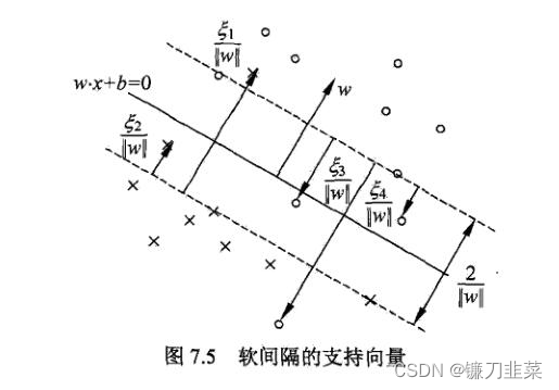
Soft interval support vector x i x_i xi Or on the boundary of the interval , Or between the interval boundary and the separation hyperplane , Or on the wrong side of the separation hyperplane .
- if α i ∗ < C \alpha_i^*<C αi∗<C, be ξ i = 0 ξ_i=0 ξi=0, Support vector x i x_i xi Right on the boundary of the gap .
- if α i ∗ = C \alpha_i^*=C αi∗=C, 0 < ξ i < 1 0<ξ_i<1 0<ξi<1, The classification is correct , x i x_i xi Between the separation boundary and the separation hyperplane .
- if α i ∗ = C \alpha_i^*=C αi∗=C, ξ i = 1 ξ_i=1 ξi=1, The classification is correct , x i x_i xi Between the separation boundary and the separation hyperplane .
- if α i ∗ = C \alpha_i^*=C αi∗=C, ξ i > 1 ξ_i>1 ξi>1, be x i x_i xi On the wrong side of the separation hyperplane .
2.4 Hinge loss function
For linear support vector machine learning , The model is a separated hyperplane w ∗ ⋅ x + b ∗ = 0 w^* \cdot x + b^*=0 w∗⋅x+b∗=0 And decision function f ( x ) = s i g n ( w ∗ ⋅ x + b ∗ ) f(x)=sign(w^* \cdot x + b^*) f(x)=sign(w∗⋅x+b∗), Its learning strategy is to maximize the soft interval , The learning algorithm is convex quadratic programming .
Description of loss function : linear SVM There is another explanation for learning , That is to minimize the following objective function :
∑ i = 1 N [ 1 − y i ( w ⋅ x i + b ) ] + + λ ∣ ∣ w ∣ ∣ 2 \sum_{i=1}^N[1−y_i(w\cdot x_i+b)]_++λ||w||^2 i=1∑N[1−yi(w⋅xi+b)]++λ∣∣w∣∣2
The... Of the objective function 1 This is an empirical risk , function L ( y ( w ⋅ x + b ) ) = [ 1 − y ( w ⋅ x + b ) ] + L(y(w\cdot x+b))=[1−y(w\cdot x+b)]_+ L(y(w⋅x+b))=[1−y(w⋅x+b)]+ be called Hinge loss function (hinge loss), Subscript “+” Represents the following positive function
[ z ] + = { z , z > 0 0 , z ≤ 0 [z]_+=\left\{\begin{matrix} z, & z>0\\ 0, & z\le 0 \end{matrix}\right. [z]+={ z,0,z>0z≤0
That is to say , When the sample point ( x i , y i ) (x_i,y_i) (xi,yi) Is correctly classified and the function interval ( Certainty ) y i ( w ⋅ x i + b ) y_i(w\cdot x_i+b) yi(w⋅xi+b) Greater than 1 when , The loss is 0, Otherwise the loss is 1 − y i ( w ⋅ x i + b ) 1−y_i(w\cdot x_i+b) 1−yi(w⋅xi+b).
The... Of the objective function 2 The term is a coefficient of λ λ λ Of w Of L 2 L_2 L2 norm , It's a regularization term .
Theorem : Linear support vector machine primitive optimization problem :
min w , b , ξ 1 2 ∣ ∣ w ∣ ∣ 2 + C ∑ i = 1 N ξ i \min_{w,b,ξ} \frac{1}{2}||w||^2 + C\sum_{i=1}^N ξ_i w,b,ξmin21∣∣w∣∣2+Ci=1∑Nξi
s . t . y i ( w ⋅ x i + b ) ⩾ 1 − ξ i , i = 1 , 2 , . . . , N s.t. y_i(w\cdot x_i + b)⩾1−ξ_i, i=1,2,...,N s.t.yi(w⋅xi+b)⩾1−ξi,i=1,2,...,N
ξ i ⩾ 0 , i = 1 , 2 , . . . , N ξ_i⩾0, i=1,2,...,N ξi⩾0,i=1,2,...,N
Equivalent to optimization problem min w , b ∑ i = 1 N [ 1 − y i ( w ⋅ x i + b ) ] + + λ ∣ ∣ w ∣ ∣ 2 \min_{w,b} \sum_{i=1}^N[1−y_i(w\cdot x_i+b)]_++λ||w||^2 w,bmini=1∑N[1−yi(w⋅xi+b)]++λ∣∣w∣∣2.
The graph of hinge loss function is shown in the figure below , The horizontal axis is the function interval y ( w ⋅ x + b ) y(w\cdot x + b) y(w⋅x+b), The vertical axis is the loss . Because the function is shaped like a hinge , So it's called hinge loss function .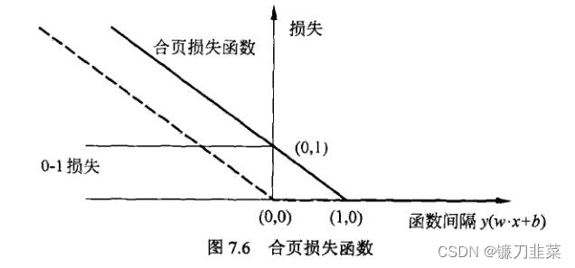
The picture also shows 0-1 Loss function , It can be considered as the real loss function of binary classification problem , The hinge loss function is 0-1 The upper bound of the loss function . because 0-1 Losses are not continuously differentiable , Direct optimization is difficult , It can be said that linear SVM It's optimization 0-1 The upper bound of loss ( Hinge loss ) The objective function . At this time, the upper bound loss is also called the proxy loss function (surrogate loss function).
The dotted line in the figure shows the loss of the sensor [ − y i ( w ⋅ x i ) + b ] + [−y_i(w\cdot x_i)+b]_+ [−yi(w⋅xi)+b]+. The loss when the sample is correctly classified is 0, Otherwise − y i ( w ⋅ x i ) + b −y_i(w\cdot x_i)+b −yi(w⋅xi)+b. by comparison , Hinge loss should not only be classified correctly , And be sure , Loss is 0, In other words, the hinge loss function has higher requirements for learning .
Content sources :
[1] 《 Statistical learning method 》 expericnce
[2] https://www.cnblogs.com/liaohuiqiang/p/10980066.html
边栏推荐
- NGUI-UILabel
- College entrance examination composition, high-frequency mention of science and Technology
- On valuation model (II): PE index II - PE band
- idm服务器响应显示您没有权限下载解决教程
- BGP actual network configuration
- Apache installation problem: configure: error: APR not found Please read the documentation
- Preorder, inorder and postorder traversal of binary tree
- OSPF exercise Report
- Vxlan 静态集中网关
- Financial data acquisition (III) when a crawler encounters a web page that needs to scroll with the mouse wheel to refresh the data (nanny level tutorial)
猜你喜欢

Epp+dis learning path (1) -- Hello world!

What is an esp/msr partition and how to create an esp/msr partition

leetcode刷题:二叉树22(二叉搜索树的最小绝对差)

Upgrade from a tool to a solution, and the new site with praise points to new value

leetcode刷题:二叉树23(二叉搜索树中的众数)
EPP+DIS学习之路(1)——Hello world!

Multi row and multi column flex layout
数据库系统原理与应用教程(011)—— 关系数据库

Cookie
Attack and defense world ----- summary of web knowledge points
随机推荐
leetcode刷题:二叉树22(二叉搜索树的最小绝对差)
On valuation model (II): PE index II - PE band
Niuke website
<No. 9> 1805. Number of different integers in the string (simple)
Completion report of communication software development and Application
Tutorial on the principle and application of database system (011) -- relational database
Error in compiling libssl
数据库系统原理与应用教程(009)—— 概念模型与数据模型
Session
Attack and defense world ----- summary of web knowledge points
牛客网刷题网址
ps链接图层的使用方法和快捷键,ps图层链接怎么做的
In the small skin panel, use CMD to enter the MySQL command, including the MySQL error unknown variable 'secure_ file_ Priv 'solution (super detailed)
Epp+dis learning path (1) -- Hello world!
VSCode的学习使用
leetcode刷题:二叉树26(二叉搜索树中的插入操作)
Using stack to convert binary to decimal
leetcode刷题:二叉树21(验证二叉搜索树)
The left-hand side of an assignment expression may not be an optional property access. ts(2779)
数据库系统原理与应用教程(010)—— 概念模型与数据模型练习题