On valuation model (II): PE index II - PE band

1： This article mainly introduces a niche valuation index ——PE Band; 

2： This paper mainly explains the concept , The model is also built by the author ;

3： The main data of this paper are through Tushare(ID：444829) Financial big data platform interface acquisition ;

4： I hope to build a trading system , The principle is to share only dry goods . More modules will be updated later , But the leisure time after work and study is limited , Please understand that the update speed is slow ;

5： The assumptions and viewpoints in this paper are based on the author's insight into the model and data , If you have different opinions, please leave a message at any time ;

6： Model implementation based on python3.8;

Catalog

1. introduction  

1.1 PE Band brief introduction

2. PE Band The irrationality and problems of

2.1 Normal distribution hypothesis

2.2 Technical analysis assumptions

2.3  Parameters

2.4  The human nature

3. PE Band Reconstruction and its significance

4. Code implementation

5. PE Band Exhibition

6. answer

---

1. introduction  

         I saw such an article before ：

One of the most favorite valuation indicators for institutional investors   Index treasure recently launched an index function ：PE Band( as well as PB Band、PS Band), This indicator is a favorite of institutional investors ... -  Snowball (xueqiu.com)

        The author searched this website ：

          What .. what , Nobody even wrote . But on second thought C There are not many financial writers like the author , Go to the mixed traffic of snowball headlines . But how many people can understand the codes put on the snowball , Finally, the author chose C standing , By the way, I can also visit other people's code masterpieces .

         Don't talk too much nonsense , Experts are far away and near , Since no one has written , Open it right now .

1.1 PE Band brief introduction

         Simply put, it's the brin line version PE indicators , The idea is mean reversion . Others have written in great detail in this article , Those who haven't seen this indicator can read it .

        I don't know how you feel after reading ; Investors who have seen and used this indicator before can also exchange their experience . All in all , The author believes that although this indicator is good or bad, it also has great defects .

        Please see Figure 1 , This is according to the link in the article PE Band Make the channel line , selection 250 Day moving range , The black line is actual PE, The red line and the green line are  band, Orange and purple are  band, The blue line is PE mean value . Then we just follow the yellow line to sell , Touch the green line or purple line to buy , It can be said that it has been tried repeatedly , There is a lot to be gained under the long air .

                                                             Figure 1 ：PE Band  Trading opportunity on

  Then next is the same picture ：

                                                              Figure 2 ： Trend forecast 【1】

at present PE In the past 250 Days low , What do you think of this stock after PE What is the trend ：

A: Rising above the red line

B: Between the orange line and the green line, there was a flat shake

C: Fall below the green line , Drop and fall

D: Too little information is given , Unable to judge

（ The answer will be announced at the end of the article ）

2. PE Band The irrationality and problems of

2.1 Normal distribution hypothesis

        Quote a sentence from that article ： " according to “3sigma The laws of ”,PE The fluctuation range of does not exceed up and down 3 The probability of times the standard deviation is 99.73%, therefore , We set this PE Band In theory , Basically, it can cover all PE value ".

        This is the first question ——PE Band Made the assumption that the stock price obeys the normal distribution , This is obviously unreasonable . The author mentioned very early that the distribution of stock prices is strange , If we calculate with normal distribution, it is undoubtedly easy to fall into the trap .

2.2 Technical analysis assumptions

        PE Band The data used is completely historical data , To put it bluntly, it is a kind of alternative Bollinger line . from PE From the perspective of index calculation formula ,PE The direction of the index is the same as that of the stock price in a financial reporting period , If we use short-term moving average as band, It directly degenerates into a brin line . I don't know how many readers trade on the brin line , Are you happy ？

2.3  Parameters

        Mentioned in this article Band What kind of Band, It is calculated based on the standard deviation of the past time 3σ band, Is it reasonable to calculate with the standard deviation of this period ？ In fact, the author is Choice This indicator is also available in the database , And many parameters can be customized , But then Choice Not every investor has paid services , both Choice this Band Style I don't like .

        Figure 3 ：Choice On Database PE Band( Data sources ：Choice database )

         Last , How to guarantee PE The index is reasonable ？ The author wrote about PE Indicators mentioned in the article PE Indicators are very vulnerable to earnings manipulation , If you currently use PE Indicators are biased , Then whether the calculated result is reliable ？

2.4  The human nature

        At the end of the article , Let's see the picture again （ The conditions are the same as those in Figure 1 ）：

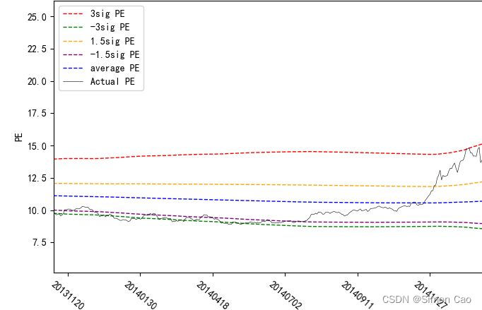
                                                          Figure 4 ： Trend forecast 【2】

at present PE It is at the high level in the past , What do you think of this stock after PE What is the trend ：

A: Continue to rise and break through the red line

B: Fall back to the green line

C: High sideways

 D: Too little information is given , Unable to judge

（ The answer will be announced at the end of the article ）

3. PE Band Reconstruction and its significance

         According to the unreasonable factors listed above, whether there is an effective solution ？ It's easy to solve for distribution , Just use a more reasonable distribution calculation Band The interval is fine . But others are hard , Maybe for biased PE Indicators we can also eliminate unreasonable factors through financial means ; But for human nature , For technical analysis, the assumption is PE Band A natural defect , At least the author can't solve it at present . If someone has good ideas, please send a private message or leave a message .

4. Code implementation

        Below, the author takes the Shanghai Composite Index as an example , Build your own PE Band For your reference . The author selected the data Tushare Financial big data interface , Register an account and you can use your own Token Request data , Very simple and convenient , Save the author from the trouble of reptiles . The website is as follows ：Tushare Big data community

        Import module first , Drawing mainly depends on matplotlib and seaborn：

import matplotlib.pyplot as plt
import seaborn as sns
import numpy as np
import tushare as ts
import pandas as pd

         Request data , The range is selected as Shanghai Stock Index 12 Year to year PE data , except PE Support in addition ttm PE,PB Equal index , Readers can read Tushare The technical documents of are set by ourselves （ Daily quotation request parameters ：Tushare Big data community ）

df = pro.index_dailybasic(ts_code=”000001.SH", start_date="20120101", end_date="20220620", fields='trade_date, pe')

        Next, let's look at the distribution ：

final_dis = np.array(df["pe"])
sns.kdeplot(final_dis)

plt.axvline(np.average(final_dis), label='mean {:.3f}'.format(np.average(final_dis)), linestyle='-.', color='r')
plt.axvline(np.median(final_dis)+np.std(final_dis)*3, label="+3Xstd {:.3f}".format(np.median(final_dis)), linestyle=':', color='g')
plt.axvline(np.median(final_dis)-np.std(final_dis)*3, label="-3Xstd {:.3f}".format(np.median(final_dis)), linestyle=':', color='g')
plt.legend()
plt.title("Distribution from 2012-2022")
plt.show()

Let's take a look at the evidence in Shanghai PE Distribution , It is not difficult to find that it is a strange shape . The author marked the normal distribution with a green dotted line 3σ Location , It is obvious that when in PE Very low period , At least you won't encounter negative 3σ Line , When the market is in a period of excitement, it is easy to overshoot the positive 3σ, Shanghai is close 10 Year of PE The average is now （ By the end of this year 6 month 20 Japan ） yes 13.4 about .

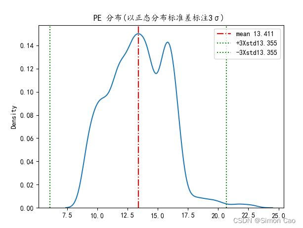
                                           Figure 5 ： The Shanghai composite index 20120101-20220620 PE Distribution

         because Band Including the upper and lower tracks , The orbital calculation here is a function , Convenient to call later . The author intends to show only two tracks ：3 Times and 1.5 times σ Of , namely multiple The ginseng 3 and 1.5. as for band The upper and lower tracks use the distribution standardization formula ： 

def sig_calc(data, multiple):
    sig = np.std(data["pe"])
    mean = np.average(data["pe"])
    probably = norm.cdf(multiple) * 100
    positive = np.percentile(data["pe"], probably)
    negative = np.percentile(data["pe"], 100 - probably)
    sig_left_tail = (mean - negative) / sig
    sig_right_tail = (positive - mean) / sig
    return sig_left_tail, sig_right_tail
    
sig_three = sig_calc(df, 3)  # 3 Sigma
sig_ahalf = sig_calc(df, 1.5) # 1.5 Sigma

         among , The following two lines are the key , According to the uniqueness of the distribution of Shanghai Stock Exchange, it reverses from the probability Band Track position , It's transformation PE Band Key steps （ It's a little similar to the hypothesis test P-value and Z value , Are the same concept , But the author uses probability to deduce on the special distribution Z value ）.

probably = norm.cdf(multiple) * 100 
positive = np.percentile(data["pe"], probably)
negative = np.percentile(data["pe"], 100 - probably)

         Get function Return Out of sig_left_tail（ Lower rail ）, sig_right_tail（ Upper rail ） After that, things will be much simpler , Set a moving range , Take the data of this decade as Band In the form of . The rest is similar to the brin line , Let's not go into details .

def lines_data(df, move_average):
    sig_three = sig_calc(df, 3)  #  The first number is the left tail 
    sig_ahalf = sig_calc(df, 1.5)

    negative_three, positive_three = [], []
    negative_ahalf, positive_ahalf = [], []
    mean_value = []
    print(sig_ahalf)
    for i in range(len(df["pe"][move_average:])):
        if np.average(df["pe"][i:move_average + i]) != None:
            stdiv = np.std(df["pe"][i:move_average + i])
            negative_three.append(np.average(df["pe"][i:move_average + i]) - sig_three[0] * stdiv)
            positive_three.append(np.average(df["pe"][i:move_average + i]) + sig_three[1] * stdiv)
            negative_ahalf.append(np.average(df["pe"][i:move_average + i]) - sig_ahalf[0] * stdiv)
            positive_ahalf.append(np.average(df["pe"][i:move_average + i]) + sig_ahalf[1] * stdiv)
            mean_value.append(np.average(df["pe"][i:move_average + i]))
        else:
            negative_three.append(None)
            positive_three.append(None)
            negative_ahalf.append(None)
            positive_ahalf.append(None)
            mean_value.append(None)
    lst = {"negative_three": negative_three,
           "positive_three": positive_three,
           "negative_ahalf": negative_ahalf,
           "positive_ahalf": positive_ahalf,
           "average": mean_value
           }
    lines = pd.DataFrame(lst)
    return lines

         Function return lines Namely Band Data of upper and lower tracks , The rest is to show them all on the map , It's all basic operations , You can choose to use it according to your preferences matplotlib perhaps Seaborn drawing , I used matplotlib：

def plot_generator(df, lines, move_average):
    plt.figure(figsize=(16, 5))
    plt.plot(df["trade_date"][move_average:], lines["positive_three"], linewidth=1, color="r", linestyle="--", label="3sig PE")
    plt.plot(df["trade_date"][move_average:], lines["negative_three"], linewidth=1, color="g", linestyle="--", label="-3sig PE")
    plt.plot(df["trade_date"][move_average:], lines["positive_ahalf"], linewidth=1, color="orange", linestyle="--",
             label="1.5sig PE")
    plt.plot(df["trade_date"][move_average:], lines["negative_ahalf"], linewidth=1, color="purple", linestyle="--",
             label="-1.5sig PE")
    plt.plot(df["trade_date"][move_average:], lines["average"], linewidth=1, color="blue", linestyle="--",
             label="average PE")
    plt.plot(df["trade_date"][move_average:], df["pe"][move_average:], linewidth=0.4, color="black", linestyle="-", label="PE")
    plt.xticks(df["trade_date"][move_average::50], rotation=320) 
    plt.xlabel("date")
    plt.ylabel("PE")
    plt.legend()
    plt.show()

5. PE Band Exhibition

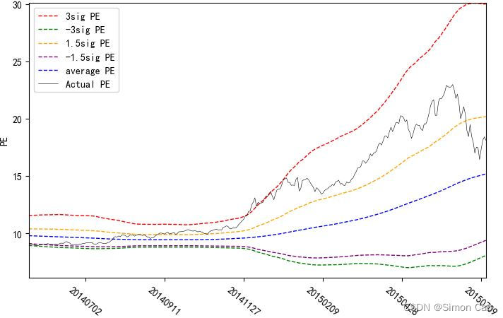
                                          Figure 6 ： The Shanghai composite index PE Band（200 Days moving standard deviation ）

         You can see , Shanghai stock index on track （1.5σ） The yellow line is sensitive in most cases , In many periods, as long as you encounter the yellow line, you will experience a decline . And the green line （3σ） Under the orbit, the reaction is relatively slow , There are many times, although they hit the green line off the track, they also fell endlessly . But overall , Short term moving average makes Band Become unreliable .

         Or you can lengthen the cycle , For example, the following figure is calculated with three years as the moving interval Band：

                                         Figure 7 ： The Shanghai composite index PE Band（720 Days moving standard deviation ）

         Looking at the long cycle ,PE When you encounter the green line, you can be sure that it is in the bottom area of the valuation , At this time, buying is very cost-effective from the perspective of long-term investment ; When PE The yellow line indicates that it is on the high side , You can choose to sell some of your positions ; When you hit the red line , This is very dangerous in the long term . in general , If you are a long-term investor, this is also a lazy stock selection method .

        The author believes that long-term PE band It has high reference value . But only for reference , It is necessary to combine the professional judgment of analysts , Don't forget the author mentioned before PE Band The shortcomings of .

6. answer

The first question is , Trend forecast 【1】C: Fall below the green line , Drop and fall

  The second question is , Trend forecast 【2】A: Continue to rise and break through the red line

  I wonder if you guessed right ？

About human nature ：

"It's going down this much already, can't go any lower."

"It's gone this high already, I gonna possibly go lower." 

"It's 3$, how much can I loose?"

-- Peter Lynch

         As mentioned in the previous article ,PE Indicators are far from as simple as they seem , I don't know after reading the author's two issues PE Does the indicator make you realize a different PE indicators . I will continue to share other interesting and useful valuation methods when I have the opportunity . If you don't abandon , We stand together through the storm .