当前位置:网站首页>[statistical learning methods] learning notes - improvement methods
[statistical learning methods] learning notes - improvement methods
2022-07-07 12:26:00 【Sickle leek】
Statistical learning methods learning notes —— How to improve
How to improve (boosting) It's a common statistical learning method , It is widely used and effective . In the classification problem , It changes the weight of training samples , Learn multiple classifiers , These classifiers are combined linearly , Improve the performance of classification . (1) Introduce boosting Methodological ideas and representative boosting Algorithm AdaBoost
(2) Through training error analysis AdaBoost Why can we improve learning accuracy
(3) Explain from the perspective of forward distribution addition model AdaBoost
(4) The last part is about boosting More specific examples of methods ——boosting tree( Ascension tree )
1. How to improve AdaBoost Algorithm
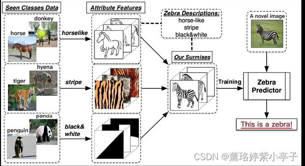
boosting The basic idea :**boosting Based on such an idea : For a complex task , The judgment is obtained by combining the judgment of multiple experts , It's better than any of the experts alone .** It's actually “ The Three Stooges , Zhuge Liang at the top ” The truth .
Strong to learn : In probability approximation correct (probably approximately correct,PAC) In the framework of learning , A concept , If there is a polynomial learning algorithm that can learn it , And the accuracy is very high , Then call this concept strongly learnable .
Weak can learn : A concept , If there is a polynomial learning algorithm that can learn it , The correct rate of learning is only slightly better than random guess , Then it is called weak learnable .
Strong learnable and weak learnable :Schapire It is proved that strong learnability and weak learnability are equivalent , in other words , stay PAC Under the framework of learning , A concept is strongly learnable if and only if it is weakly learnable .
From weak learning to strong learning : Can be “ Weak learning ” Upgrade to “ Strong learning ”, Weak learning algorithms are usually much easier than strong learning algorithms . How to implement improvement , It is called the problem to be solved when developing promotion methods . Many lifting algorithms have been proposed , The most representative AdaBoost.
** The lifting method starts from the weak learning algorithm , Learn over and over again , We get a series of weak classifiers ( Also known as base classifier ), Then combine these weak classifiers , Make a strong classifier .** Most of the promotion methods are to change the probability distribution of training data ( Weight distribution of training data ), For different training data distribution , Call weak learning algorithm to learn a series of weak classifiers . Here are two questions .
(1) How to change the weight or probability distribution of training data in each round
(2) How to combine weak classifiers into a strong classifier
For the two problems mentioned above ,AdaBoost The approach is
(1) Improve the weight of samples that have been incorrectly classified by the previous round of weak classifiers , Reduce the weight of those samples that are correctly classified . thus , The data that didn't get the right classification , Due to the increase of weight, it has received greater attention from the later round of weak classifiers .
(2) A weighted majority vote , Increase the weight of the weak classifier with small classifier error , Make it a big part in the voting , Reduce the weight of weak classifier with large classification error , Make it play a smaller role in voting .
Algorithm :AdaBoost
Input : Training data set T = ( x 1 , y 1 ) , ( x 2 , y 2 ) , . . . , ( x N , y N ) T=(x_1,y_1),(x_2,y_2),...,(x_N,y_N) T=(x1,y1),(x2,y2),...,(xN,yN), among x i ∈ X ⊆ R n , y i ∈ { − 1 , + 1 } x_i∈\mathcal{X}⊆R^n,y_i\in \{−1,+1\} xi∈X⊆Rn,yi∈{ −1,+1}. Weak learning algorithm .
Output : The final classifier G ( x ) G(x) G(x)
(1) Initialize the weight distribution of training data
D 1 = ( w 11 , . . . , w 1 i , . . . , w 1 N ) , w 1 i = 1 N , i = 1 , 2 , . . . , N D_1=(w_{11},...,w_{1i},...,w_{1N}), w_{1i}=\frac{1}{N}, i=1,2,...,N D1=(w11,...,w1i,...,w1N),w1i=N1,i=1,2,...,N
here It is assumed that the data has a uniform weight distribution , Each sample has the same learning function in the base classifier .
(2) Yes m=1,2,…,M
(a) The weight distribution is D m D_m Dm Training data learning , Get the base classifier G m ( x ) : X → { + 1 , − 1 } G_m(x):\mathcal{X}→\{+1,−1\} Gm(x):X→{ +1,−1}
(b) Calculation G m ( x ) G_m(x) Gm(x) The classification error rate on the training set
e m = ∑ i = 1 N P ( G m ( x i ) ≠ y i ) = ∑ i = 1 N w m i I ( G m ( x i ) ≠ y i ) = ∑ G m ( x i ) ≠ y i w m i e_m=\sum_{i=1}^N P(G_m(x_i)≠y_i)=\sum_{i=1}^N w_{mi} I(G_{m}(x_i)\ne y_i)=\sum_{G_m(x_i)\ne y_i}w_{mi} em=i=1∑NP(Gm(xi)=yi)=i=1∑NwmiI(Gm(xi)=yi)=Gm(xi)=yi∑wmi
here , w m i w_{mi} wmi It means the first one m In the middle of the round i The weight of each instance , ∑ i = 1 N w m i = 1 \sum_{i=1}^N w_{mi}=1 ∑i=1Nwmi=1, indicate G m ( x ) G_m(x) Gm(x) The classification error rate on the weighted training data set is G m ( x ) G_m(x) Gm(x) Sum of the weights of the misclassified samples .
(c) Calculation G m ( x ) G_m(x) Gm(x) The coefficient of : α m = 1 2 log 1 − e m e m α_m=\frac{1}{2} \log{\frac{1−e_m}{e_m}} αm=21logem1−em, Logarithm is natural logarithm . α m α_m αm Express G m ( x ) G_m(x) Gm(x) Importance in the final classifier . e m ⩽ 0.5 e_m⩽0.5 em⩽0.5 when α m ⩾ 0 α_m⩾0 αm⩾0, and α m α_m αm With e m e_m em Decrease and increase , The smaller the classification error, the greater the role of the base classifier in the final classifier .
(d) Update the weight distribution of the training set , Prepare for the next round
D m + 1 = ( w m + 1 , 1 , . . . , w m + 1 , i , . . . , w m + 1 , N ) D_{m+1}=(w_{m+1,1},...,w_{m+1,i},...,w_{m+1,N}) Dm+1=(wm+1,1,...,wm+1,i,...,wm+1,N)
w m 1 , i = { w m i z m e − α m , G m ( x i ) = y i w m i z m e α m , G m ( x i ) ≠ y i w_{m_1, i}=\left\{\begin{matrix} \frac{w_{mi}}{z_m}e^{-\alpha _m}, & G_{m}(x_i)=y_i \\ \frac{w_{mi}}{z_m}e^{\alpha _m}, & G_{m}(x_i)\ne y_i \end{matrix}\right. wm1,i={ zmwmie−αm,zmwmieαm,Gm(xi)=yiGm(xi)=yi
Z m = ∑ i = 1 N w m i e x p ( − α m y i G m ( x i ) ) Z_m=\sum_{i=1}^N w_{mi}exp(−α_my_iG_m(x_i)) Zm=i=1∑Nwmiexp(−αmyiGm(xi))
among Z m Z_m Zm For normalization factor .
The weight of misclassified samples becomes larger , The weight of correctly classified samples is reduced , The two-phase comparison is magnified e 2 α m = 1 − e m e m e^{2\alpha_m}=\frac{1−e_m}{e_m} e2αm=em1−em times .
(3) Construct a linear combination of base classifiers
f ( x ) = ∑ m = 1 M α m G m ( x ) f(x)=\sum_{m=1}^M α_mG_m(x) f(x)=m=1∑MαmGm(x)
The final classifier is
G ( x ) = s i g n ( f ( x ) ) G(x)=sign(f(x)) G(x)=sign(f(x))
Be careful α m α_m αm The sum is not 1.
2. AdaBoost Training error analysis of algorithm
AdaBoost The most basic property is that it can continuously reduce training errors in the learning process .
Theorem 8.1(AdaBoost The error margin of training ):AdaBoost The training error bound of the final classifier is
1 N ∑ i = 1 N I ( G ( x i ) ≠ y i ) ⩽ 1 N ∑ i e x p ( − y i f ( x i ) ) = ∏ m Z m \frac{1}{N}\sum_{i=1}^{N} I(G(x_i)≠y_i)⩽\frac{1}{N}\sum_i exp(−y_if(x_i))=\prod_m Z_m N1i=1∑NI(G(xi)=yi)⩽N1i∑exp(−yif(xi))=m∏Zm
Theorem 8.2 ( Dichotomous problem AdaBoost The error margin of training )
∏ m = 1 M Z m = ∏ m = 1 M [ 2 e m ( 1 − e m ) ] = ∏ m = 1 M 1 − 4 γ m 2 ≤ e x p ( − 2 ∑ m = 1 M γ m 2 ) \prod_{m=1}^M Z_m=\prod_{m=1}^{M} [2\sqrt{e_m(1−e_m)}]=\prod_{m=1}^{M}\sqrt{1−4\gamma_m^2} \le exp(−2\sum_{m=1}^{M}\gamma_m^2) m=1∏MZm=m=1∏M[2em(1−em)]=m=1∏M1−4γm2≤exp(−2m=1∑Mγm2)
here γ m = 1 2 − e m \gamma_m=\frac{1}{2}−e_m γm=21−em.
inference 8.1: If there is γ > 0 \gamma>0 γ>0, For all m Yes γ m ⩾ γ \gamma_m⩾\gamma γm⩾γ, be
1 N ∑ i = 1 N I ( G ( x i ) ≠ y i ) ⩽ e x p ( − 2 M γ 2 ) \frac{1}{N}\sum_{i=1}^{N} I(G(x_i)≠y_i)⩽exp(−2M\gamma^2) N1i=1∑NI(G(xi)=yi)⩽exp(−2Mγ2)
This indicates that under these conditions AdaBoost The training error of is decreasing exponentially , This nature is certainly attractive .
Different from some early promotion methods ,AdaBoost It's adaptive , That is, it can adapt to the respective training error rates of weak classifiers . This is also the origin of its name ,Ada yes Adaptive Abbreviation .
3. AdaBoost Explanation of algorithm
It can be said that AdaBoost The algorithm is an additive model 、 The loss model is exponential 、 Class II classification learning method when the learning algorithm is forward distribution algorithm .
3.1 Forward distribution algorithm
Consider the additive model (additive model)
f ( x ) = ∑ m = 1 M β m b ( x ; γ m ) f(x)=\sum_{m=1}^M β_m b(x; γ_m) f(x)=m=1∑Mβmb(x;γm)
among , b ( x ; γ m ) b(x; \gamma_m) b(x;γm) Is the base function , γ m \gamma_m γm Is the parameter of the base function , β m \beta_m βm Is the coefficient of the basis function .
In a given training set and loss function L ( y , f ( x ) ) L(y,f(x)) L(y,f(x)) Under the condition of , Learn the addition model f ( x ) f(x) f(x) It becomes an empirical risk minimization problem, that is, the minimization of loss function :
min β m , γ m ∑ i = 1 N L ( y i , ∑ m = 1 M β m b ( x i ; γ m ) ) \min_{β_m,γ_m}\sum_{i=1}^N L(y_i,\sum_{m=1}M β_mb(x_i; γ_m)) βm,γmmini=1∑NL(yi,m=1∑Mβmb(xi;γm))
Usually this is a complex optimization problem . The idea of forward step-by-step algorithm to solve this optimization problem is : From front to back , We're only going to learn one basis function and its coefficients at each step , The objective function of optimization is approached step by step , Then the complexity of optimization can be simplified . Optimize the following losses in each step :
min β , γ ∑ i = 1 N L ( y i , β b ( x i ; γ ) ) \min_{β,γ}\sum_{i=1}^N L(y_i,βb(x_i; γ)) β,γmini=1∑NL(yi,βb(xi;γ))
Given the training data set T = ( x 1 , y 1 ) , ( x 2 , y 2 ) , . . . , ( x N , y N ) T=(x_1,y_1),(x_2,y_2),...,(x_N,y_N) T=(x1,y1),(x2,y2),...,(xN,yN), among x i ∈ X ⊆ R n , y i ∈ { − 1 , + 1 } x_i∈\mathcal{X}⊆R^n,y_i\in \{−1,+1\} xi∈X⊆Rn,yi∈{ −1,+1}. Loss function L ( y , f ( x ) ) L(y,f(x)) L(y,f(x)) And the set of basis functions { b ( x ; γ ) } \{b(x; \gamma)\} { b(x;γ)}, Learn the addition model f ( x ) f(x) f(x) The forward step algorithm of is as follows :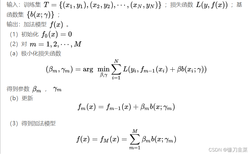
such , The forward step algorithm will simultaneously solve from m = 1 m=1 m=1 To M All the parameters β m \beta_m βm , γ m \gamma_m γm The optimization problem is simplified to solve each problem step by step β m \beta_m βm , γ m \gamma_m γm Optimization problem .
3.2 Forward distribution algorithm and AdaBoost
From the forward step-by-step algorithm, we can deduce AdaBoost, Use theorem to describe this relationship .
Theorem 8.3:AdaBoost The algorithm is a special case of forward step-by-step addition algorithm . At this time , The model is an additive model composed of basic classifiers , The loss function is exponential .
4. Ascension tree
Lifting tree is a kind of lifting method based on classification tree or regression tree . The ascension tree is considered One of the best performance methods in statistical learning .
4.1 Ascension tree model
The lifting method is actually based on the additive model ( That is, the linear combination of basis functions ) And the forward step-by-step algorithm . The lifting method based on decision tree is called lifting tree (boosting tree). For classification problems, the decision tree is a binary classification tree , For regression problems, the decision tree is a binary regression tree .
The promotion tree model can be expressed as the addition model of decision tree :
f M ( x ) = ∑ m = 1 M T ( x ; θ m ) f_M(x)=\sum_{m=1}^M T(x; θ_m) fM(x)=m=1∑MT(x;θm)
among , T ( x ; θ m ) T(x;θ_m) T(x;θm) Represents a decision tree , θ m θ_m θm For the parameters of the decision tree , M M M For the number of trees .
4.2 Lifting tree algorithm
The lifting tree algorithm adopts the forward step-by-step algorithm . First determine the initial lift tree f 0 ( x ) = 0 f_0(x)=0 f0(x)=0, The first m The model of step is
f m ( x ) = f m − 1 ( x ) + T ( x ; θ m ) f_m(x)=f_{m-1}(x)+T(x;\theta_m) fm(x)=fm−1(x)+T(x;θm)
among , f m − 1 ( x ) f_{m-1}(x) fm−1(x) For the current model , The parameters of the next decision tree are determined by empirical risk minimization θ m θ_m θm.
θ ^ m = a r g min θ m ∑ i = 1 N L ( y i , f m − 1 ( x i ) + T ( x i ; θ m ) ) \hat{\theta}_m=arg\min_{θ_m}\sum_{i=1}{N} L(y_i,f_{m−1}(x_i)+T(x_i;θ_m)) θ^m=argθmmini=1∑NL(yi,fm−1(xi)+T(xi;θm))
Because the linear combination of trees can fit the training data well , Even if the relationship between input and output in the data is complex . So the lifting tree is a high-function learning algorithm .
Learning algorithm of lifting tree : Next, we discuss the lifting tree learning algorithm for different problems , The main difference is that the loss function used is different . Include Use the classification problem of index loss , Use the regression problem of square loss , as well as Use the general decision problem of general loss .
For dichotomies , Just put the AdaBoost The base classifier of is limited to a binary classification tree , It can be said that the lifting tree algorithm at this time is Adaboost A special case of the algorithm .
The ascending tree of the regression problem , Will input space X Divided into J Disjoint regions R 1 , R 2 , . . . , R J R_1,R_2,...,R_J R1,R2,...,RJ, And determine the output constant in each region c j c_j cj, Then the tree can be expressed as
T ( x i ; θ ) = ∑ j = 1 J c j I ( x ∈ R j ) T(x_i;θ)=\sum_{j=1}^J c_j I(x\in R_j) T(xi;θ)=j=1∑JcjI(x∈Rj)
among , Parameters θ = { ( R 1 , c 1 ) , ( R 2 , c 2 ) , . . . , ( R J , c J ) } θ=\{(R_1,c_1),(R_2,c_2),...,(R_J,c_J)\} θ={ (R1,c1),(R2,c2),...,(RJ,cJ)} Represents the region division of the tree and the constants on each region . J J J Is the complexity of the regression tree, that is, the number of leaf nodes .
The regression problem lifting tree uses the following forward step-by-step Algorithm :
f 0 ( x ) = 0 f m ( x ) = f m − 1 ( x ) + T ( x ; θ m ) , m = 1 , 2 , . . . , M f M ( x ) = ∑ i = 1 M T ( x ; θ m ) f_0(x)=0 \\\\ f_m(x) = f_{m−1}(x)+T(x;θ_m), m=1,2,...,M \\\\ f_M(x)=\sum_{i=1}^{M} T(x;θ_m) f0(x)=0fm(x)=fm−1(x)+T(x;θm),m=1,2,...,MfM(x)=i=1∑MT(x;θm)
In the second step of the forward step-by-step algorithm m Step , Given the current model f m − 1 ( x ) f_{m−1}(x) fm−1(x), Demand solution
θ ^ m = a r g min θ m ∑ i = 1 N L ( y i , f m − 1 ( x i ) + T ( x i ; θ m ) ) \hat{\theta}_m=arg\min_{θ_m}\sum_{i=1}^{N} L(y_i,f_{m−1}(x_i)+T(x_i;θ_m)) θ^m=argθmmini=1∑NL(yi,fm−1(xi)+T(xi;θm))
obtain θ ^ m \hat{\theta}_m θ^m, That is to say m The parameters of a tree .
When square loss is used , L ( y , f ( x ) ) = ( y − f ( x ) ) 2 L(y, f(x))=(y-f(x))^2 L(y,f(x))=(y−f(x))2, Its loss becomes
L ( y , f m − 1 ( x ) + T ( x ; θ m ) ) = [ y − f m − 1 ( x ) − T ( x ; θ m ) ] 2 = [ r − T ( x ; θ m ) ] 2 L(y, f_{m−1}(x)+T(x;θ_m))=[y−f_{m−1}(x)−T(x;θ_m)]^2=[r−T(x;θ_m)]^2 L(y,fm−1(x)+T(x;θm))=[y−fm−1(x)−T(x;θm)]2=[r−T(x;θm)]2
here , r = y − f m − 1 ( x ) r=y−f_{m−1}(x) r=y−fm−1(x), Is the residual of the current model fitting data . therefore , For the lifting tree algorithm of regression problem , Simply fit the residuals of the current model .
Algorithm : The lifting tree algorithm of regression problem 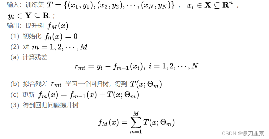
4.3 Gradient rise
The lifting tree uses the addition model and the forward step-by-step algorithm to realize the optimization process of learning , When the loss function is a square loss function and an exponential loss function , Each step of optimization is very simple , But for the general loss function , Often every step of optimization is not so easy . To address this issue ,Freidman Gradient lifting method is proposed (gradient boosting) Algorithm , It's using The approximate method of the steepest descent method , The key is Using the negative gradient of the loss function The value in the current model − [ ∂ L ( y , f ( x i ) ) ∂ f ( x i ) ] f ( x ) = f m − 1 ( x ) -[\frac{\partial L(y,f(x_i))}{\partial f(x_i)}]_{f(x)=f_{m-1}(x)} −[∂f(xi)∂L(y,f(xi))]f(x)=fm−1(x) As an approximation of the residuals in the lifting tree algorithm for regression problems , Fit a regression tree .
Algorithm : Gradient lifting algorithm 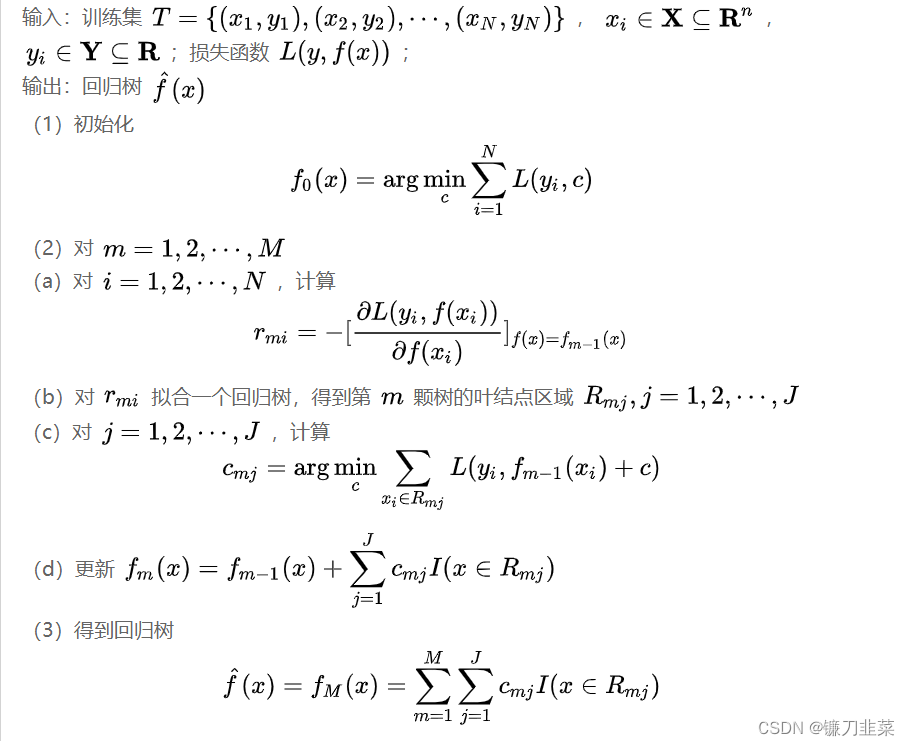
summary
- The promotion method is a statistical learning method that promotes the weak learning algorithm to the strong learning algorithm .
- AdaBoost The model is a linear combination of weak classifiers .
- AdaBoost The feature of the algorithm is to learn one basic classifier each time through iteration .
- AdaBoost Each iteration can reduce its classification error rate on the training data set .
- Lifting tree is a lifting method based on classification tree or regression tree .
Add
Gradient Boosting
Gradient Boosting Machine( abbreviation GBM), from Freidman Put forward , It's a kind of An algorithm based on gradient lifting .
classical AdaBoost The algorithm can only deal with the binary classification learning task with exponential loss function ( Of course , Now there are those who can handle multiple classification or regression tasks AdaBoost Algorithm variation ), and Gradient Boosting Various learning tasks can be handled by setting different differentiable loss functions ( classification 、 Return to 、 Sort, etc ), The scope of application is greatly expanded .
AdaBoost For outliers (outlier) Is more sensitive , and Gradient Boosting By introducing bagging thought 、 Methods such as adding regular terms can effectively resist the noise in the training data , Better robustness .
Gradient Boosting The basic idea of , Take the negative gradient as a measure of learning mistakes in the previous round , In the next round of learning, we can correct the mistakes made in the previous round by fitting the negative gradient . The key question here is : Why can we correct the last round of errors by fitting the negative gradient ?Freidman The answer is : The gradient of function space falls .
GBDT
Gradient lifting tree , Often referred to as GBDT(Gradient Boosting Decision Tree), Or is it GBT(Gradient Boosting Tree),GTB(Gradient Tree Boosting ),GBRT(Gradient Boosting Regression Tree),MART(Multiple Additive Regression Tree).GBDT It has been widely used in practical business , It plays an important role in machine learning algorithm .GBDT It's using CART The regression tree in
When solving classification problems ,GBDT The common loss functions are : Index loss ( Return to Adaboost)、 Negative logarithmic loss . Index loss is easily affected by outliers , And it can only be used for binary classification problems , therefore sklearn in GradientBoostingClassifier The default loss function of is the latter .
In solving the problem of return ,GBDT The common loss functions are : Mean square error loss 、 Absolute loss 、Huber Loss and quantile loss . about Huber Loss and quantile loss , Often used for robust regression , It can reduce the influence of outliers on the loss function , contrary , The loss of mean square deviation is easily affected by outliers .
XGBoost
XGBoost It's right GBDT The extended implementation of , Not only is it more efficient in speed , And the algorithm derivation has also been improved . The main differences between the two are as follows :
- GBDT With CART Regression tree as a base learner ,XGBoost It supports gbtree、dart and gblinear Three basic learning devices . among , The first two are tree based models ,dart And I think about it dropout thought ,gblinear Is a linear model , This is the time XGBoost It's equivalent to taking L1 and L2 Logical regression of regularized terms ( Classification problem ) Or linear regression ( The return question ).
- GBDT We only use the first derivative information when we optimize ,XGBoost Second order Taylor expansion of the cost function is carried out , First and second derivatives are used at the same time . By the way ,XGBoost The tool supports custom cost functions , As long as the function is first-order and second-order differentiable .
More fundamentally ,GBDT Mainly for loss L ( y , F ) L(y,F) L(y,F) About F F F Find gradient , The regression tree is used to fit the negative gradient ;XGBoost Mainly for loss L ( y , F ) L(y,F) L(y,F) Second order Taylor expansion , Then find the analytical solution , With analytical solution o b j obj obj As a standard , Greedy search split Whether the tree o b j obj obj better , More direct . - XGBoost Regular terms are added to the cost function , To control the complexity of the model . The regular term contains the number of leaf nodes in the tree 、 Output on each leaf node score Of L2 The sum of the squared magnitudes . from bias-variance tradeoff perspective , Regular terms reduce the value of the model variance, Make the model easier to learn , Prevent over fitting .
- XGBoost We learn from random forest , Support column sampling (column subsampling), That is, randomly select some features for learning , This not only reduces over fitting , It also reduces computation .
- There is a missing sample for the value of the feature ,XGBoost Can automatically learn its split direction .
- XGBoost Tools support parallelism . It should be noted that , Parallelism here is not tree Granularity parallelism ,XGBoost One iteration is the end of the next iteration ( The first t The cost function of the second iteration contains the preceding t-1 The predicted value of the second iteration ),XGBoost The parallelism of is on the feature granularity .
We know , One of the most time-consuming steps in learning a decision tree is to sort the values of the features ( Because we want to determine the optimal segmentation point ),XGBoost Before training , Sort the data in advance , Save as block structure , This structure is reused in subsequent iterations , Greatly reduced computation . This block Structure also makes parallelism possible : When splitting nodes , You need to calculate the gain for each feature , Finally, the feature with the largest gain is selected to split , Then the gain calculation of each feature can be opened multithreading , Achieve the goal of parallelism . - When the tree node is splitting , We need to calculate the gain of each segmentation point for each feature , That is to enumerate all possible segmentation points by greedy method . When data cannot be loaded into memory at one time or in a distributed situation , Greedy algorithms become inefficient , therefore XGBoost A parallel approximate histogram algorithm is also proposed , For efficient generation of candidate segmentation points .
- XGBoost The regression tree and GBDT What is used CART The regression tree is not consistent , The leaf node output value of the latter , Is the mean value of all sample points assigned to the leaf node , The leaf node output value of the former is calculated according to the scoring formula .
- Boosting The main concern is to reduce bias, therefore Boosting It can build strong integration based on learners with weak generalization performance ;Bagging The main concern is to reduce variance, So it's not pruning the decision tree 、 The effectiveness of neural network is more obvious .
LightGBM It is an open source library of Microsoft in recent years , Compare with XGBoost, It is faster and uses less memory .LightGBM The improvement points of the system mainly lie in the following aspects :
- Using histogram algorithm to find segmentation points , Reduce memory footprint 、 Speed up
- use Leaf-wise The way to build , Improve accuracy
- Optimization of parallel learning
- Reduce the training set (GOSS)、 Reduce features (EFB)
Content sources
[1] 《 Statistical learning method 》 expericnce
[2] https://www.cnblogs.com/liaohuiqiang/p/10980080.html
[3] 《 Statistical learning method 》 series (8)
边栏推荐
- How to connect 5V serial port to 3.3V MCU serial port?
- EPP+DIS学习之路(1)——Hello world!
- Superscalar processor design yaoyongbin Chapter 9 instruction execution excerpt
- SQL lab 1~10 summary (subsequent continuous update)
- SQL Lab (46~53) (continuous update later) order by injection
- What are the technical differences in source code anti disclosure
- About web content security policy directive some test cases specified through meta elements
- idm服务器响应显示您没有权限下载解决教程
- Unity中SmoothStep介绍和应用: 溶解特效优化
- 《通信软件开发与应用》课程结业报告
猜你喜欢
![[data clustering] realize data clustering analysis based on multiverse optimization DBSCAN with matlab code](/img/83/0652e3138b87a4741dd8261a24d1e8.png)
[data clustering] realize data clustering analysis based on multiverse optimization DBSCAN with matlab code

UP Meta—Web3.0世界创新型元宇宙金融协议
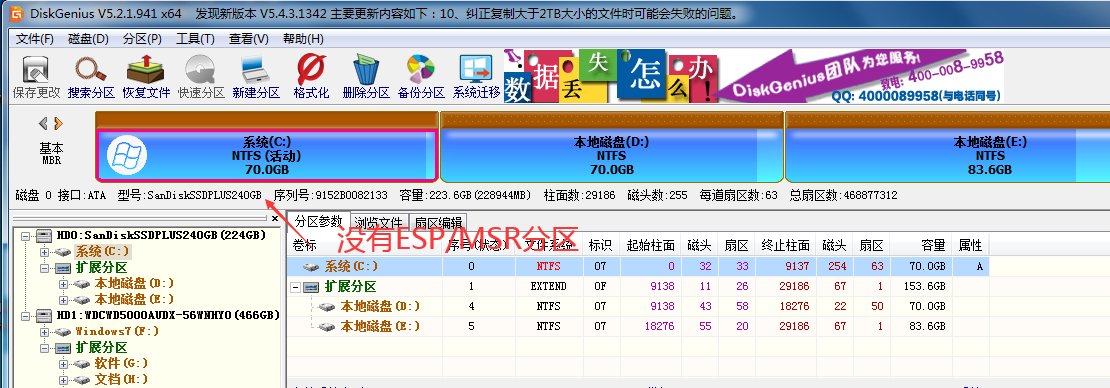
什么是ESP/MSR 分区,如何建立ESP/MSR 分区
zero-shot, one-shot和few-shot
数据库系统原理与应用教程(011)—— 关系数据库

Minimalist movie website
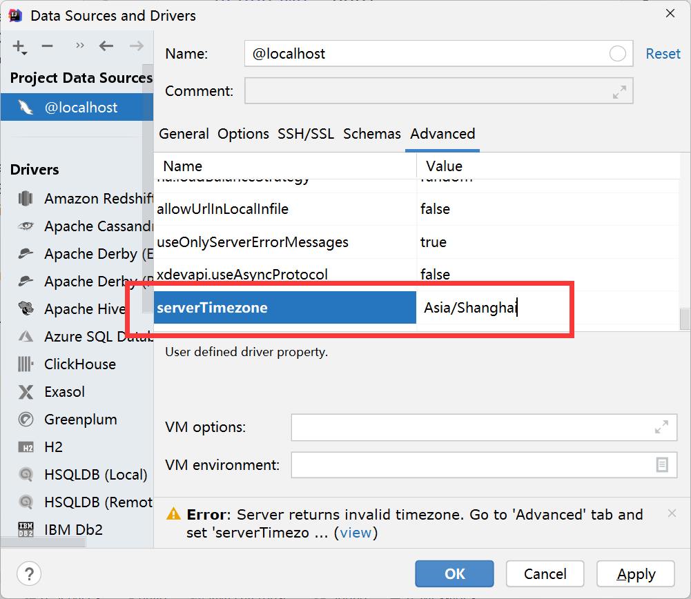
解决 Server returns invalid timezone. Go to ‘Advanced’ tab and set ‘serverTimezone’ property manually
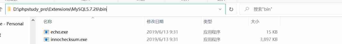
In the small skin panel, use CMD to enter the MySQL command, including the MySQL error unknown variable 'secure_ file_ Priv 'solution (super detailed)
Tutorial on principles and applications of database system (009) -- conceptual model and data model
Static routing assignment of network reachable and telent connections
随机推荐
Fleet tutorial 15 introduction to GridView Basics (tutorial includes source code)
Introduction and application of smoothstep in unity: optimization of dissolution effect
About sqli lab less-15 using or instead of and parsing
AirServer自动接收多画面投屏或者跨设备投屏
盘点JS判断空对象的几大方法
Tutorial on principles and applications of database system (009) -- conceptual model and data model
数据库系统原理与应用教程(007)—— 数据库相关概念
How to connect 5V serial port to 3.3V MCU serial port?
In the small skin panel, use CMD to enter the MySQL command, including the MySQL error unknown variable 'secure_ file_ Priv 'solution (super detailed)
如何理解服装产业链及供应链
The hoisting of the upper cylinder of the steel containment of the world's first reactor "linglong-1" reactor building was successful
gcc 编译报错
EPP+DIS学习之路(2)——Blink!闪烁!
《看完就懂系列》天哪!搞懂节流与防抖竟简单如斯~
SQL head injection -- injection principle and essence
消息队列消息丢失和消息重复发送的处理策略
Epp+dis learning road (2) -- blink! twinkle!
File upload vulnerability - upload labs (1~2)
OSPF exercise Report
Inverted index of ES underlying principle